My last post laid out the basics of the Fourier transforms, these are an integral part of vibration analysis. But in Fourier transforms, one of the big issues engineers see is that the frequencies that appear in their data do not line up well with the analysis frequency, so the signal starts to “leak” into the surrounding frequencies.
Signals rarely ever line up perfectly, but these issues can be cleared up by taking more data and applying a technique called windowing. Before we get to the solution, let’s look at the problem in more detail.
Introduction to the Problem
A Signal Without Leakage
Let’s start with a slightly modified version of where we ended the last post. We’re still sampling at 100uS, but we’ll add a small component at 2kHz. The signal we’re now analyzing is:
x(t)=sin(2π1000t)+sin(2π4000t+π/4)+0.2sin(2π2000t)
x[n]=x(nT_s )=sin(2π0.1n)+sin(2π0.4n+π/4)+0.2sin(2π0.2n)
The first 20 points look like:
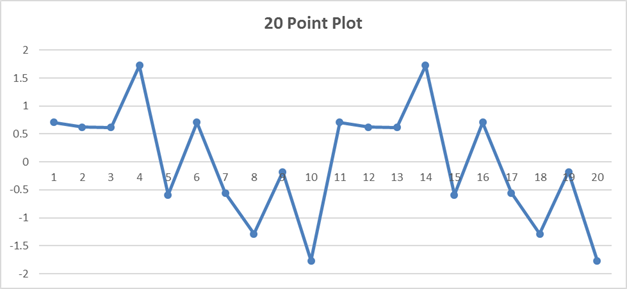
And if we take a 20 sample normalized Fourier transform we get:
|
n |
Real |
Imag |
Freq |
n |
Real |
Imag |
Freq |
|
X[0] |
0 |
j0 |
0 Hz |
X[10] |
0 |
j0 |
5.0 kHz |
|
X[1] |
0 |
j0 |
0.5 kHz |
X[11] |
0 |
j0 |
5.5 kHz |
|
X[2] |
0 |
-j0.5 |
1.0 kHz |
X[12] |
0.3536 |
j0.3536 |
6.0 kHz |
|
X[3] |
0 |
j0 |
1.5 kHz |
X[13] |
0 |
j0 |
6.5 kHz |
|
X[4] |
0 |
-j0.1 |
2.0 kHz |
X[14] |
0 |
j0 |
7.0 kHz |
|
X[5] |
0 |
j0 |
2.5 kHz |
X[15] |
0 |
j0 |
7.5 kHz |
|
X[6] |
0 |
j0 |
3.0 kHz |
X[16] |
0 |
j0.1 |
8.0 kHz |
|
X[7] |
0 |
j0 |
3.5 kHz |
X[17] |
0 |
j0 |
8.5 kHz |
|
X[8] |
0.3536 |
-j0.3536 |
4.0 kHz |
X[18] |
0 |
j0.5 |
9.0 kHz |
|
X[9] |
0 |
j0 |
4.5 kHz |
X[19] |
0 |
j0 |
9.5 kHz |
A Signal With Leakage
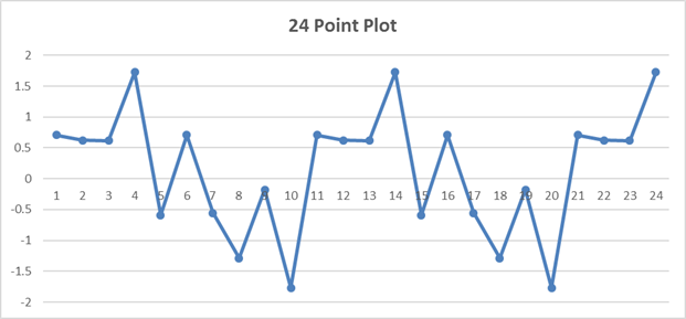
Everything looks nice and clean. Now, let’s try 24 samples. More data should be better, right? Now we get:
|
n |
Real |
Imag |
Freq (kHz) |
n |
Real |
Imag |
Freq (kHz) |
|
X[0] |
0.152825 |
j0 |
0 |
X[12] |
-0.04268 |
j0 |
5.000 |
|
X[1] |
0.178331 |
-j0.01349 |
0.417 |
X[13] |
-0.055 |
j0.057259 |
5.417 |
|
X[2] |
0.426835 |
-j0.0933 |
0.833 |
X[14] |
-0.17402 |
j0.307707 |
5.833 |
|
X[3] |
-0.17649 |
j0.108472 |
1.250 |
X[15] |
0.113483 |
-j0.24794 |
6.250 |
|
X[4] |
-0.02225 |
j0.075647 |
1.667 |
X[16] |
0.040938 |
-j0.10281 |
6.667 |
|
X[5] |
-0.05788 |
-j0.02282 |
2.083 |
X[17] |
0.020678 |
-j0.06632 |
7.083 |
|
X[6] |
0.003853 |
j0.045956 |
2.500 |
X[18] |
0.003853 |
-j0.04596 |
7.500 |
|
X[7] |
0.020678 |
j0.066323 |
2.917 |
X[19] |
-0.05788 |
j0.022816 |
7.917 |
|
X[8] |
0.040938 |
j0.102811 |
3.333 |
X[20] |
-0.02225 |
-j0.07565 |
8.333 |
|
X[9] |
0.113483 |
j0.247941 |
3.750 |
X[21] |
-0.17649 |
-j0.10847 |
8.750 |
|
X[10] |
-0.17402 |
-j0.30771 |
4.167 |
X[22] |
0.426835 |
j0.093304 |
9.167 |
|
X[11] |
-0.055 |
-j0.05726 |
4.583 |
X[23] |
0.178331 |
j0.013489 |
9.583 |
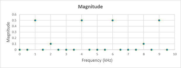
Taking more data made the image a lot less clear. We are putting in 1 kHz, 2 kHz, and 4 kHz signals, but our analysis does not directly cover those frequencies, so the frequencies “leak” into all the other frequencies.
Leakage and Windowing
To get a better picture of what leakage looks like, let’s look at the magnitude, normalized by the number of samples, for each point.
|
Sample |
Magnitude |
Freq |
Sample |
Magnitude |
Freq |
|
X[0] |
0.145 |
0 Hz |
X[12] |
0.0446 |
5.000 kHz |
|
X[1] |
0.171 |
0.417 kHz |
X[13] |
0.08 |
5.417 kHz |
|
X[2] |
0.429 |
0.833 kHz |
X[14] |
0.353 |
5.833 kHz |
|
X[3] |
0.213 |
1.250 kHz |
X[15] |
0.275 |
6.250 kHz |
|
X[4] |
0.071 |
1.667 kHz |
X[16] |
0.114 |
6.667 kHz |
|
X[5] |
0.054 |
2.083 kHz |
X[17] |
0.076 |
7.083 kHz |
|
X[6] |
0.060 |
2.500 kHz |
X[18] |
0.06 |
7.500 kHz |
|
X[7] |
0.076 |
2.917 kHz |
X[19] |
0.054 |
7.917 kHz |
|
X[8] |
0.114 |
3.333 kHz |
X[20] |
0.071 |
8.333 kHz |
|
X[9] |
0.275 |
3.750 kHz |
X[21] |
0.213 |
8.750 kHz |
|
X[10] |
0.353 |
4.167 kHz |
X[22] |
0.429 |
9.167 kHz |
|
X[11] |
0.08 |
4.583 kHz |
X[23] |
0.171 |
9.583 kHz |

Expanding the number of samples way out to 124 makes the situation more clear:
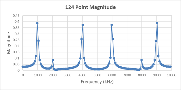
When the frequency of the signal does not exactly line up with a frequency covered by the analysis, then the signal will spill over into adjacent frequencies. Taking more data makes the frequency peaks more obvious, but we still get the leakage.
Window Functions
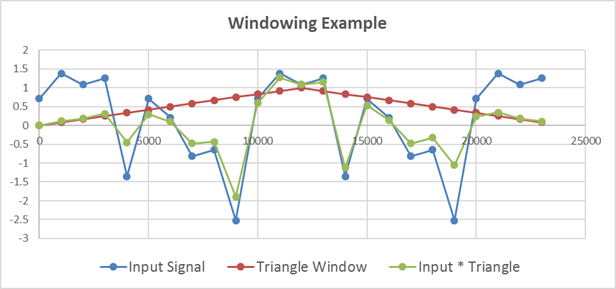
This leakage can never be completely removed, but it can be reduced by applying a window function to the signal. Windowing is a very complicated idea that is actually simple in practice. Simply multiply the window function, point by point, into your signal, and take the Fourier transform of the result.
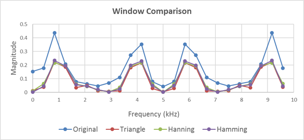
Three common window functions are the triangle, Hanning window, and Hamming window:
|
Window |
Equation |
|
Triangle |
= 2n/N for n =< N/2, = 2-2n/N for n > N/2 |
|
Hanning |
= 0.5 – 0.5 cos(2πn/(N-1)) |
|
Hamming |
= 0.54 – 0.46 cos(2πn/(N-1)) |
In this case, the windows each perform similarly, but any of these magnitudes are a much better representation of the actual signal than the transform of the unwindowed signal was.
Below, we have 3 examples of the same comparison on 20 and 28 point plots as well:
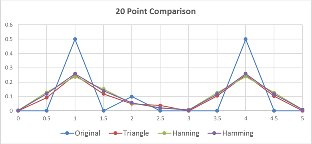
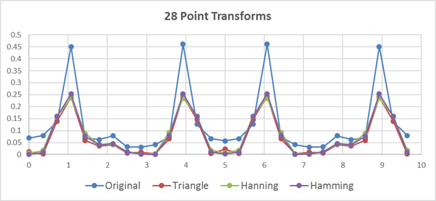
We can see from the 20 sample example that for a small, perfectly aligned set of data, the windowing makes the situation a bit worse. This makes sense as it is hard to improve on perfection. But when we start adding samples, the unwindowed data can get better or worse, while the windowed data tends to mainly get better.
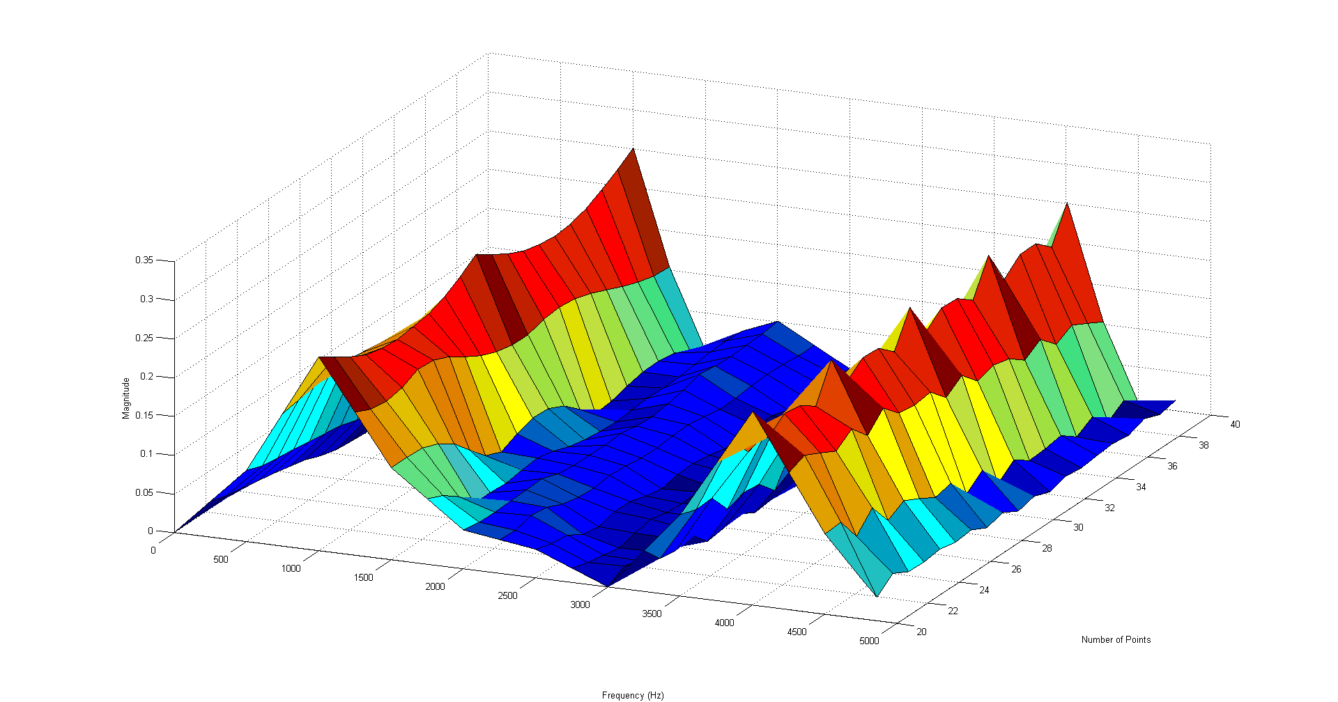
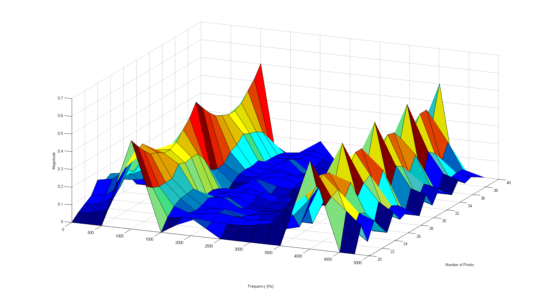
This trend is more obvious from the plots below. First, I have a 3D plot generated in MATLAB that uses the X axis (into the page) to show plots with a different number of points taken, from 20 to 40. You can see that the 1 and 4 kHz peaks bounce up and down dramatically, and the 2 kHz peak periodically disappears. To make a complicated plot clearer, the plot only shows frequencies below 5 kHz.
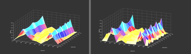
And this shows the same set of signals with a triangle window applied. Notice how the peaks improve in a much more uniform way compared to the unwindowed data:
In enDAQ's Lab Software (formerly Mide's Lab software), we use the Hanning window to clean up the data, which is especially effective in the spectrograms, where the data is divided down into smaller consecutive segments 4-1000 mS long.
The MATLAB scripts I used to generate these files are available for download below.
Example MATLAB® Scripts for Window Comparisons
These files were used to generate the graphs that appear on the blog post. You can use them to test out the calculations.
- 3D Leakage Graph
- Comparison Plots
- Window Functions
MATLAB® Scripts for Window Comparision:
Window Comparison Files (2 KB):