What’s faster, MATLAB or Python? There are a lot of forums out there comparing the two programming languages; but none seemed to give actual computation times for real analysis. This post will.
In this post we’ll test two similar MATLAB and Python scripts as they perform some basic vibration analysis. These scripts do the following:
- Load in a two column CSV
- Plot all data
- Compute and plot the moving 1 second RMS level
- Compute and plot a FFT
The MATLAB and Python functions are available to download as well as the vibration data files used in the analysis. We’ll look at data sets ranging in size from tens of thousands of points to tens of millions. For an introduction to Python, check out our article Get Started with Python: Why and How Mechanical Engineers Should Make the Switch.
MATLAB and Python Background
I’m a MATLAB guy. I’ve probably been using MATLAB for about 10 years and I must admit I love performing some “MATLAB magic.” But I’ve learned more and more about Python over the last several years as fellow engineers here at enDAQ (a division of Midé) use it to create our enDAQ Lab (formerly Slam Stick Lab) vibration analysis software package. I’ve also frequently fielded questions from customers of our enDAQ sensors (formerly Slam Stick vibration logger products) asking how to perform their vibration analysis. I’ve recommended both Python and MATLAB; but then the follow-on question is… well what’s better, MATLAB or Python?
Python
In general Python has the advantage of being free, open source, and more versatile. Their NumPy and SciPy packages have similar functions to MATLAB. Python is a pretty elegant and intuitive programming language compared to MATLAB. It was created to be a generic language that is easy to read; and they definitely succeeded with that! Python is universally accepted as the better alternative to MATLAB for other programming needs besides data analysis.
MATLAB
MATLAB, on the other hand, was developed specifically for linear algebraic operations which could make it faster for vibration analysis applications. The downside is that the language can be a little more difficult to read/understand; but MATLAB is generally considered more cleanly packaged because you get an extensive library of functions and an integrated development environment (IDE) in one. For Python you need to install extra packages and the IDE (not a major lift to do though!).
The big disadvantage of MATLAB is that it's not free, a commercial license will run you $2,150. They also charge more, typically $1,000, for additional toolboxes; and I'd recommend the signal processing toolbox for vibration analysis. Don't worry though, I didn't use any functions in that toolbox for this analysis or the ones covered in my vibration analysis basics blog. Here's a full price list of the MATLAB products. MathWorks (the makes of MATLAB) are smart with their pricing though in that they offer significantly discounted licenses to students (get the entire suite including all toolboxes for $99) and to home users ($149 for MATLAB, $45 for signal processing toolbox). So must engineering students will come out of university with a knowledge and preference for MATLAB. They then take this preference to their future employer giving MATLAB the edge.
MATLAB vs Python
There are a lot of blogs and forums out there comparing the two programming languages/platforms (here’s a relatively biased, but informative, Python vs MATLAB comparison). A coworker here at enDAQ (a division of Mide) said that its difficult to compare Python directly to MATLAB: “it’s like comparing a diesel engine to a gas one, each has unique benefits and drawbacks,” he said. Maybe because of their differences, I had trouble finding an objective comparison of performance on real data sets for the type of analysis that I, or vibration customers, would be performing. So I set out to objectively measure the difference!
The Code
MATLAB® Vibration Analysis Function:
I wanted the comparison between Python and MATLAB to be as apples-to-apples as possible. I also wanted it to be doing a useful analysis, one typical for vibration testing. I wrote the initial script in MATLAB to prompt the user for a CSV, load the CSV, and plot all data. I then perform a simple moving RMS calculation and plot this followed by a FFT of the entire data set and plot. The script times how long each of these major steps take. I’m looking at moving RMS because this gives a sense of the strength of the vibration as it moves with time. An FFT is one of the fundamental first vibration analysis steps. Check out my blog on FFTs for some more background. Writing the MATLAB script was the easy part. Here it is below. The .m file is also available for download.
|
01
02
03
04
05
06
07
08
09
10
11
12
13
14
15
16
17
18
19
20
21
22
23
24
25
26
27
28
29
30
31
32
33
34
35
36
37
38
39
40
41
42
43
44
45
46
47
48
49
50
51
52
53
54
55
56
57
58
59
60
61
|
close allclear all%Get filename and path [fname,pathname] = uigetfile('.csv','Select CSV File to Load, Plot, Compute RMS & FFT'); disp([pathname fname])%Load CSV tic %start timer data = csvread([pathname fname]); fprintf('%4.2f seconds - Time to Load Data\n',toc) %Determine variables and Display size [N,m] = size(data); t = data(:,1); %time in seconds x = data(:,2); %array of data for RMS and FFT Fs = 1/(t(2)-t(1)); fprintf('%12.0f data points\n',N)%Plot Data tic %start timer figure(1) plot(t,x) xlabel('Time (s)'); ylabel('Accel (g)'); title(fname); grid on; fprintf('%4.2f seconds - Time to Plot Data\n',toc) %Determine RMS and Plot tic %start timer w = floor(Fs); %width of the window for computing RMS steps = floor(N/w); %Number of steps for RMS t_RMS = zeros(steps,1); %Create array for RMS time values x_RMS = zeros(steps,1); %Create array for RMS values for i=1:steps range = ((i-1)*w+1):(i*w); t_RMS(i) = mean(t(range)); x_RMS(i) = sqrt(mean(x(range).^2)); end figure(2) plot(t_RMS,x_RMS) xlabel('Time (s)'); ylabel('RMS Accel (g)'); title(['RMS - ' fname]); grid on; fprintf('%4.2f seconds - Time to Compute RMS and Plot\n',toc) %Determine FFT and Plot tic freq = 0:Fs/length(x):Fs/2; %frequency array for FFT xdft = fft(x); %Compute FFT xdft = 1/length(x).*xdft; %Normalize xdft(2:end-1) = 2*xdft(2:end-1); figure(3) plot(freq,abs(xdft(1:floor(N/2)+1))) xlabel('Frequency (Hz)'); ylabel('Accel (g)'); title(['FFT - ' fname]); grid on; fprintf('%4.2f seconds - Time to Compute FFT and Plot\n',toc) |
close all
clear all

%Get filename and path
    [fname,pathname] = uigetfile('.csv','Select CSV File to Load, Plot, Compute RMS & FFT');
    disp([pathname fname])

%Load CSV
    tic %start timer
    data = csvread([pathname fname]);
    fprintf('%4.2f seconds - Time to Load Data\n',toc)

%Determine variables and Display size
    [N,m] = size(data);
    t = data(:,1); %time in seconds
    x = data(:,2); %array of data for RMS and FFT
    Fs = 1/(t(2)-t(1));
    fprintf('%12.0f data points\n',N)

%Plot Data
    tic %start timer
    figure(1)
    plot(t,x)
    xlabel('Time (s)');
    ylabel('Accel (g)');
    title(fname);
    grid on;
    fprintf('%4.2f seconds - Time to Plot Data\n',toc)

%Determine RMS and Plot
    tic %start timer
    w = floor(Fs); %width of the window for computing RMS
    steps = floor(N/w); %Number of steps for RMS
    t_RMS = zeros(steps,1); %Create array for RMS time values
    x_RMS = zeros(steps,1); %Create array for RMS values
    for i=1:steps
        range = ((i-1)*w+1):(i*w);
        t_RMS(i) = mean(t(range));
        x_RMS(i) = sqrt(mean(x(range).^2));
    end
    figure(2)
    plot(t_RMS,x_RMS)
    xlabel('Time (s)');
    ylabel('RMS Accel (g)');
    title(['RMS - ' fname]);
    grid on;
    fprintf('%4.2f seconds - Time to Compute RMS and Plot\n',toc)

%Determine FFT and Plot
    tic
    freq = 0:Fs/length(x):Fs/2; %frequency array for FFT
    xdft = fft(x); %Compute FFT
    xdft = 1/length(x).*xdft; %Normalize
    xdft(2:end-1) = 2*xdft(2:end-1);
    figure(3)
    plot(freq,abs(xdft(1:floor(N/2)+1)))
    xlabel('Frequency (Hz)');
    ylabel('Accel (g)');
    title(['FFT - ' fname]);
    grid on;
    fprintf('%4.2f seconds - Time to Compute FFT and Plot\n',toc)
Python Vibration Analysis Function:
The hard part was to write an equivalent script in Python. I had never written any Python scripts as of two days ago. I was pleasantly surprised with how easily I was able to “translate” this MATLAB script into Python. There are a ton of resources online, I found this NumPy for MATLAB users tutorial particularly helpful. The Pyhon script is provided below. The length of the scripts are virtually the same; the Python script is a couple lines longer to load in the necessary libraries. The .py file is available for download.
|
01
02
03
04
05
06
07
08
09
10
11
12
13
14
15
16
17
18
19
20
21
22
23
24
25
26
27
28
29
30
31
32
33
34
35
36
37
38
39
40
41
42
43
44
45
46
47
48
49
50
51
52
53
54
55
56
57
58
59
60
61
62
63
64
65
66
67
|
import matplotlib.pyplot as pltimport numpy as npfrom scipy.fftpack import fftimport tkinter as tkfrom tkinter import filedialogimport time#Prompt user for fileroot = tk.Tk()root.withdraw()file_path = filedialog.askopenfilename(filetypes=[("Two Column CSV","*.csv")])print(file_path)#Load Data (assumes two column arraytic = time.clock()t, x = np.genfromtxt(file_path,delimiter=',', unpack=True)toc = time.clock()print("Load Time:",toc-tic)#Determine variablesN = np.int(np.prod(t.shape))#length of the arrayFs = 1/(t[1]-t[0]) #sample rate (Hz)T = 1/Fs;print("# Samples:",N)#Plot Datatic = time.clock()plt.figure(1) plt.plot(t, x)plt.xlabel('Time (seconds)')plt.ylabel('Accel (g)')plt.title(file_path)plt.grid()toc = time.clock()print("Plot Time:",toc-tic)#Compute RMS and Plottic = time.clock()w = np.int(np.floor(Fs)); #width of the window for computing RMSsteps = np.int_(np.floor(N/w)); #Number of steps for RMSt_RMS = np.zeros((steps,1)); #Create array for RMS time valuesx_RMS = np.zeros((steps,1)); #Create array for RMS valuesfor i in range (0, steps): t_RMS[i] = np.mean(t[(i*w):((i+1)*w)]); x_RMS[i] = np.sqrt(np.mean(x[(i*w):((i+1)*w)]**2)); plt.figure(2) plt.plot(t_RMS, x_RMS)plt.xlabel('Time (seconds)')plt.ylabel('RMS Accel (g)')plt.title('RMS - ' + file_path)plt.grid()toc = time.clock()print("RMS Time:",toc-tic)#Compute and Plot FFTtic = time.clock()plt.figure(3) xf = np.linspace(0.0, 1.0/(2.0*T), N/2)yf = fft(x)plt.plot(xf, 2.0/N * np.abs(yf[0:np.int(N/2)]))plt.grid()plt.xlabel('Frequency (Hz)')plt.ylabel('Accel (g)')plt.title('FFT - ' + file_path)toc = time.clock()print("FFT Time:",toc-tic)plt.show() |
import matplotlib.pyplot as plt
import numpy as np
from scipy.fftpack import fft
import tkinter as tk
from tkinter import filedialog
import time

#Prompt user for file
root = tk.Tk()
root.withdraw()
file_path = filedialog.askopenfilename(filetypes=[("Two Column CSV","*.csv")])
print(file_path)

#Load Data (assumes two column array
tic = time.clock()
t, x = np.genfromtxt(file_path,delimiter=',', unpack=True)
toc = time.clock()
print("Load Time:",toc-tic)

#Determine variables
N = np.int(np.prod(t.shape))#length of the array
Fs = 1/(t[1]-t[0])  #sample rate (Hz)
T = 1/Fs;
print("# Samples:",N)

#Plot Data
tic = time.clock()
plt.figure(1)
plt.plot(t, x)
plt.xlabel('Time (seconds)')
plt.ylabel('Accel (g)')
plt.title(file_path)
plt.grid()
toc = time.clock()
print("Plot Time:",toc-tic)

#Compute RMS and Plot
tic = time.clock()
w = np.int(np.floor(Fs)); #width of the window for computing RMS
steps = np.int_(np.floor(N/w)); #Number of steps for RMS
t_RMS = np.zeros((steps,1)); #Create array for RMS time values
x_RMS = np.zeros((steps,1)); #Create array for RMS values
for i in range (0, steps):
    t_RMS[i] = np.mean(t[(i*w):((i+1)*w)]);
    x_RMS[i] = np.sqrt(np.mean(x[(i*w):((i+1)*w)]**2));
plt.figure(2)
plt.plot(t_RMS, x_RMS)
plt.xlabel('Time (seconds)')
plt.ylabel('RMS Accel (g)')
plt.title('RMS - ' + file_path)
plt.grid()
toc = time.clock()
print("RMS Time:",toc-tic)

#Compute and Plot FFT
tic = time.clock()
plt.figure(3)
xf = np.linspace(0.0, 1.0/(2.0*T), N/2)
yf = fft(x)
plt.plot(xf, 2.0/N * np.abs(yf[0:np.int(N/2)]))
plt.grid()
plt.xlabel('Frequency (Hz)')
plt.ylabel('Accel (g)')
plt.title('FFT - ' + file_path)
toc = time.clock()
print("FFT Time:",toc-tic)
plt.show()
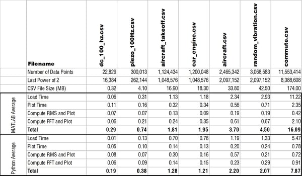
Vibration Data Files
We go through 7 different vibration data sets in this comparison. Most of these recording are explained in a little more depth on our vibration analysis basics blog post. All data was captured using our enDAQ sensors and I exported the data to CSV. The first two recordings are from a 60 second recording with the sensor on a shaker table vibrating at a constant 10g, 100 Hz sinusoidal input. One file is from the MEMS accelerometer sampling at 400 Hz; the other is from the piezoelectric accelerometer sampling at 5,000 Hz.
We also look at a recording file from the sensor sampling at 10,000 Hz on the shaker being excited with a random vibration exposure profile in accordance with MIL-STD-810G. Two recordings look at vibrations on an aircraft. One (aircraft.csv) is from a recording with the enDAQ sensor on the outside of a plane with a 2,500 Hz sample rate (can’t share too much about the application). The second recording (aircraft_takeoff.csv) is when I mounted a sensor to the seat in front of me during takeoff on a commercial flight and sampled at 2,000 Hz. My wife wasn’t too pleased with that test…
The final two recordings are looking at data of my car’s (2008 Saab 93 2.0T) engine. The first recording (car_engine.csv) is part of our how-to video series that has more information. The second and largest dataset (commute.csv) is when I mounted the sensor to my engine and record the vibrations during my morning commute which included going on the highway. I live close by so it’s only a 20 minute recording but I was sampling at 10,000 Hz so there are over 11 million data points.
Test Setup – Computer and Software Used
I did all the testing on my work computer which is a Dell Precision T3610. It has an Intel Xeon 3.00 GHz processor and 8 GB of RAM. The operating system is Windows 7 Professional 64-bit. The MATLAB I’m using is R2014b, 64-bit. I downloaded and ran Python 3.5.2 64-bit, NumPy 1.11.1, and SciPy 0.18.0.
All data and scripts were saved on my C drive for the testing. I ran each twice and took the average. I made sure the two times were comparable between the tests. I had a fair number of programs running (MATLAB, Chrome, Outlook, Excel, Visio, and Word); but I kept all programs open during both tests (Python and MATLAB) to keep things consistent.
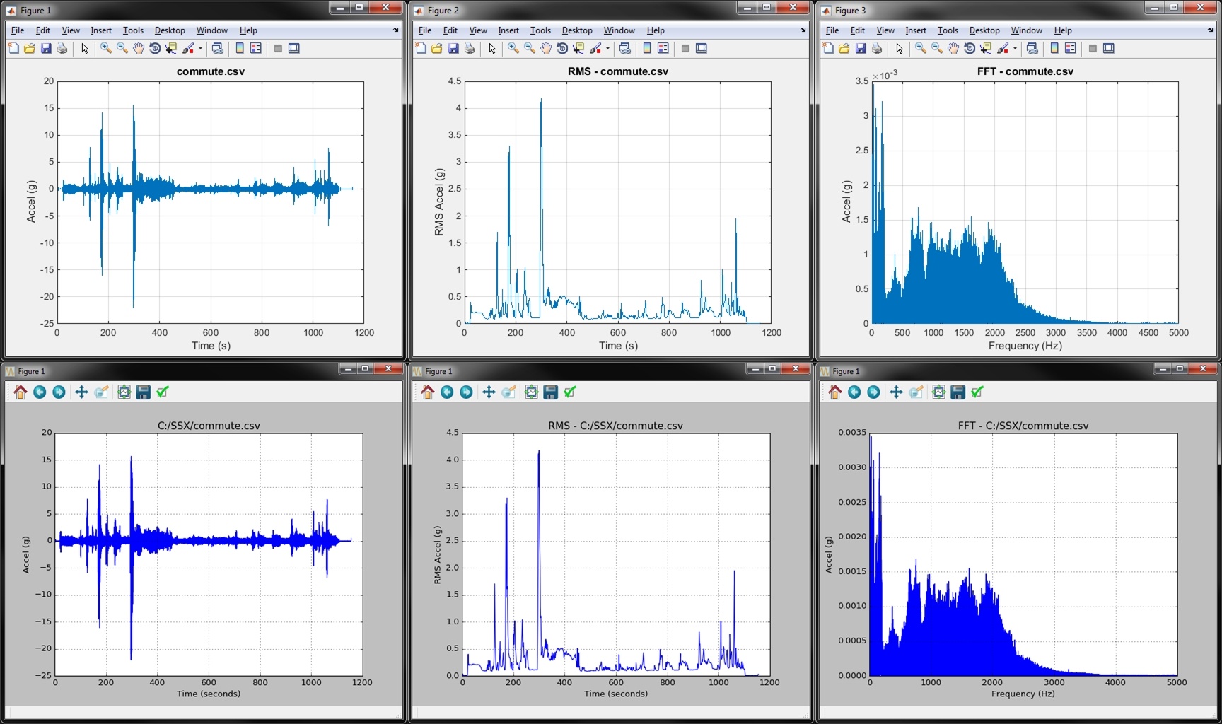
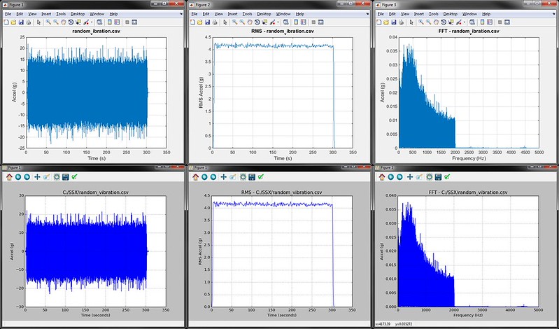
The Plots Gallery
Click through below to see the vibration analysis example plots generated from the two scripts. The top are from MATLAB, the bottom from Python. From left to right, the whole data set is plotted, then the moving RMS, then a FFT of the entire data set. You can see that both MATLAB and Python get to the same place; but the question is how quickly did they get there?
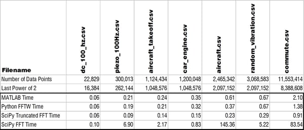
The Results
Below is a table with all times listed in seconds comparing how quickly MATLAB and Python performed the main functions.
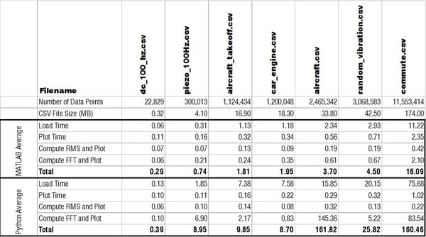
Loading a CSV
My immediate question was why the heck is MATLAB able to load in a CSV to memory so much faster than Python?! Check out a log-log plot of the time difference; MATLAB is consistently an order of magnitude faster! I couldn’t understand how/why this is the case so I restarted my computer to see if MATLAB was doing something clever with using memory that wasn’t ever really cleared. But the results after restarting my computer were comparable.
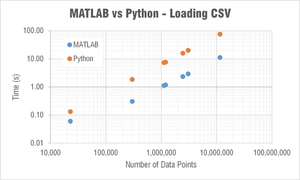
Side note: When I first did this test I was using the numpy.loadtxt() function. One of the engineers here recommended the numpy.genfromtxt() function which was three times faster! Still though not nearly as fast as MATLAB. The comparison plots and table show data when using the faster genfromtxt() function.
Plotting and Computing Moving RMS
Python did an equivalent job plotting and computing RMS as MATLAB. This was relatively expected from what I had read and I was happy with Python's performance here! One note though is that MATLAB plot windows are a little more richer with information and options for customization. Apparently IPython is an interactive Python shell that's great for similar plotting customization to MATLAB. Here's a nice tutorial on IPython.
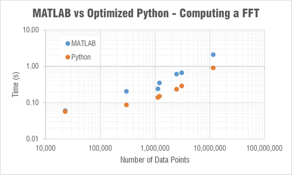
Computing FFT
The next major question though was what the heck is going on with SciPy’s FFT computation times!?
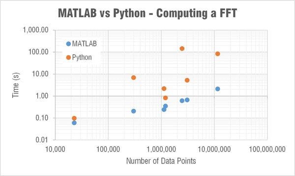
MATLAB’s FFT function has a relatively linear dependency on the array’s length. This is expected as they state:
The execution time of an FFT algorithm depends on the transform length. It is fastest when the transform length is a power of two, and almost as fast when the transform length has only small prime factors. It is typically slower for transform lengths that are prime or have large prime factors. Time differences, however, are reduced to insignificance by modern FFT algorithms such as those used in MATLAB. Adjusting the transform length for efficiency is usually unnecessary in practice.
The computation time in SciPy’s FFT function was barely linear and very weird… For example it took 30 times longer to compute a FFT for an array length 2,465,342 than one of length 3,068,583. Let me say that again, it took 30 times longer to compute an FFT on an array with over a half a million less data points! I reran this test many times to see if something strange was happening on my computer; but it is repeatable. When I showed this to Mide's FFT expert Pete (he recently wrote a post that goes a bit deeper into the math behind FFTs) he immediately began writing a couple scripts to look a little deeper into this. Subscribe to our blog if you’re interested in what he finds out.
Optimizing Python to Beat MATLAB
At first glance, this testing wasn't a great look for Python. But I did some digging and spoke to a couple of the engineers here on ways to improve the Python performance.
Two suggestions were made:
- Use the pandas data analysis library's read_csv() function for importing
- Truncate the array to the last power of 2 for FFT calculation
Optimized Python Code
It only added a couple lines of code to optimize the vibration analysis script. The major differences being another library imported and a line or two to calculate the last power of 2 and truncate the array. Here it is below.
|
01
02
03
04
05
06
07
08
09
10
11
12
13
14
15
16
17
18
19
20
21
22
23
24
25
26
27
28
29
30
31
32
33
34
35
36
37
38
39
40
41
42
43
44
45
46
47
48
49
50
51
52
53
54
55
56
57
58
59
60
61
62
63
64
65
66
67
68
69
70
71
72
73
|
import matplotlib.pyplot as pltimport pandas as pdimport numpy as npfrom scipy.fftpack import fftimport tkinter as tkfrom tkinter import filedialogimport time#Prompt user for fileroot = tk.Tk()root.withdraw()file_path = filedialog.askopenfilename(filetypes=[("Two Column CSV","*.csv")])print(file_path)#Load Data (assumes two column arraytic = time.clock()df = pd.read_csv(file_path,delimiter=',',header=None,names=["time","data"])t = df["time"]x = df["data"]toc = time.clock()print("Load Time:",toc-tic)#Determine variablesN = np.int(np.prod(t.shape))#length of the arrayN2 = 2**(N.bit_length()-1) #last power of 2Fs = 1/(t[1]-t[0]) #sample rate (Hz)T = 1/Fs;print("# Samples:",N)print("Next power of 2:",N2)#Plot Datatic = time.clock()plt.figure(1) plt.plot(t, x)plt.xlabel('Time (seconds)')plt.ylabel('Accel (g)')plt.title(file_path)plt.grid()toc = time.clock()print("Plot Time:",toc-tic)#Compute RMS and Plottic = time.clock()w = np.int(np.floor(Fs)); #width of the window for computing RMSsteps = np.int_(np.floor(N/w)); #Number of steps for RMSt_RMS = np.zeros((steps,1)); #Create array for RMS time valuesx_RMS = np.zeros((steps,1)); #Create array for RMS valuesfor i in range (0, steps): t_RMS[i] = np.mean(t[(i*w):((i+1)*w)]); x_RMS[i] = np.sqrt(np.mean(x[(i*w):((i+1)*w)]**2)); plt.figure(2) plt.plot(t_RMS, x_RMS)plt.xlabel('Time (seconds)')plt.ylabel('RMS Accel (g)')plt.title('RMS - ' + file_path)plt.grid()toc = time.clock()print("RMS Time:",toc-tic)#Compute and Plot FFTtic = time.clock()plt.figure(3) N = N2 #truncate array to the last power of 2xf = np.linspace(0.0, 1.0/(2.0*T), N/2)yf = fft(x, n = N)plt.plot(xf, 2.0/N * np.abs(yf[0:np.int(N/2)]))plt.grid()plt.xlabel('Frequency (Hz)')plt.ylabel('Accel (g)')plt.title('FFT - ' + file_path)toc = time.clock()print("FFT Time:",toc-tic)plt.show() |
import matplotlib.pyplot as plt
import pandas as pd
import numpy as np
from scipy.fftpack import fft
import tkinter as tk
from tkinter import filedialog
import time

#Prompt user for file
root = tk.Tk()
root.withdraw()
file_path = filedialog.askopenfilename(filetypes=[("Two Column CSV","*.csv")])
print(file_path)

#Load Data (assumes two column array
tic = time.clock()
df = pd.read_csv(file_path,delimiter=',',header=None,names=["time","data"])
t = df["time"]
x = df["data"]
toc = time.clock()
print("Load Time:",toc-tic)

#Determine variables
N = np.int(np.prod(t.shape))#length of the array
N2 = 2**(N.bit_length()-1) #last power of 2
Fs = 1/(t[1]-t[0])  #sample rate (Hz)
T = 1/Fs;
print("# Samples:",N)
print("Next power of 2:",N2)

#Plot Data
tic = time.clock()
plt.figure(1)
plt.plot(t, x)
plt.xlabel('Time (seconds)')
plt.ylabel('Accel (g)')
plt.title(file_path)
plt.grid()
toc = time.clock()
print("Plot Time:",toc-tic)

#Compute RMS and Plot
tic = time.clock()
w = np.int(np.floor(Fs)); #width of the window for computing RMS
steps = np.int_(np.floor(N/w)); #Number of steps for RMS
t_RMS = np.zeros((steps,1)); #Create array for RMS time values
x_RMS = np.zeros((steps,1)); #Create array for RMS values
for i in range (0, steps):
    t_RMS[i] = np.mean(t[(i*w):((i+1)*w)]);
    x_RMS[i] = np.sqrt(np.mean(x[(i*w):((i+1)*w)]**2));
plt.figure(2)
plt.plot(t_RMS, x_RMS)
plt.xlabel('Time (seconds)')
plt.ylabel('RMS Accel (g)')
plt.title('RMS - ' + file_path)
plt.grid()
toc = time.clock()
print("RMS Time:",toc-tic)

#Compute and Plot FFT
tic = time.clock()
plt.figure(3)
N = N2 #truncate array to the last power of 2
xf = np.linspace(0.0, 1.0/(2.0*T), N/2)
yf = fft(x, n = N)
plt.plot(xf, 2.0/N * np.abs(yf[0:np.int(N/2)]))
plt.grid()
plt.xlabel('Frequency (Hz)')
plt.ylabel('Accel (g)')
plt.title('FFT - ' + file_path)
toc = time.clock()
print("FFT Time:",toc-tic)
plt.show()
Overview of Optimized Results
Below is a table that has the Python computation times with the updated/optimized script. There is a significant improvement!
Loading a CSV
I had no issue installing the pandas library which claims "to be the fundamental high-level building block for doing practical, real world data analysis in Python." The plot below shows the loading times. Without pandas, MATLAB was loading a CSV 10 times faster than Python; now Python is twice as fast as MATLAB!
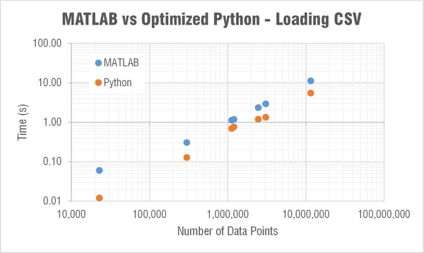
The naysayers out there (myself included) will say that in MATLAB you wouldn't need to use CSVs and could use their impressive binary MAT file format. And that's true, you should try to be using MAT files when in MATLAB. If I load the MAT file with the same data as that 11.5 million point commute.csv file, MATLAB loads it in 0.7 seconds. A noticeable improvement over the 11 seconds it takes when loading the CSV. The file itself is also much smaller (54 vs 174 MB). But SciPy has a few functions for loading and saving MAT files (scipy.io). And Python loads that same MAT file in around 0.7 seconds as well. So it seems that MATLAB can't claim faster loading times over Python even when using their own file format!
As Jake and TheBlackCat pointed out in the comments (thank you!), loading a CSV is not a great way to go if you're loading large data files. And I definitely agree; I used that in this testing because it's a little more well-known to the non-technical folks out there. But if you'll be loading large data sets you should be using a binary file format like HDF5 or UFF58.
Truncating the FFT
I was a bit hesitant to truncate the array length to the last power of 2 because I felt that this wasn't going to be an apples-to-apples comparison to MATLAB. I also didn't like missing the end of an array which may have had some different frequency content that a FFT would have been able to pick up. I thought about zero-padding the array to increase to the next power of 2; but the added zeros can smear the FFT peaks. And with the type of data files I'm used to on enDAQ sensors (high sample rate and battery life equals millions of data points) I don't care too much about missing the end of a recording in a FFT (just do a spectrogram to capture it). I'm much more concerned with reducing the amplitude of my frequency components though. I use that information to generate power spectral densities for determining the vibration response of my system.
In the MATLAB plot below the FFT results are compared when truncating or zero padding the aircraft takeoff data. You can see that truncating leads to pretty similar amplitudes when compared to an unmodified array. But check out the results when zero padding the array; it significantly reduces the FFT amplitude. I wouldn't recommend zero padding when you need to draw conclusions from the amplitude of your FFT (which would be most vibration analysis applications). If you're only interested in the frequencies themselves then zero padding is preferred because the frequency resolution would be improved and all data is still analyzed. All that being said, there are a ton of different ways to compute a FFT and you can do scaling and windowing with zero padding to get comparable results. I'll punt that discussion for another day though (subscribe to our blog if you're interested in finding out more). For the purpose of optimizing Python's FFT computation time to compete with MATLAB, just truncate. If you are worried about missing data then compute two FFTs for each half of the file and/or compute and plot a spectrogram.
So I went with truncating. When the array was truncated to the last power of two Python is able to compute an FFT in roughly half the time compared to MATLAB! If I do this same truncation in the MATLAB script though the computation times are comparable. I wouldn't recommend doing the truncation for MATLAB because it doesn't need it (who really cares about 1 second faster on an 11 million data point array at the price of missing data?). Python, on the other hand, clearly needs this truncation. Truncating allows Python to be as much as 1,000 times faster!
Forget about trying to compute the FFT without truncating if you get a prime number as the array length. Let's look at the aircraft take off data as an example again. It's length is 1,124,434 and Python (specifically SciPy) computes the FFT in 2 seconds (MATLAB does it in 0.2). If we truncate down to 1,048,576 (2^20) it computes in 0.14 seconds. Now if we truncate down 5 data points to the prime number 1,124,429 the FFT computes in... well I don't know, I gave up after waiting 10 minutes! Meanwhile MATLAB computed the FFT of this in 0.5 seconds.
Truncated FFT Gallery
Click through the plots below (MATLAB on the left, Python on the right) to see how reducing the FFT length affects the amplitude. There are definitely small differences but they're pretty close. So again, if you're in Python it's worthwhile to truncate arrays before computing a FFT. MATLAB doesn't seem to need this and would be the preferred option if you don't feel comfortable truncating and potentially missing data.
Python's PyFFTW Algorithm
After I initially posted this blog several folks commented (thank you!) and suggested I check out the pyFFTW Python library that uses the FFTW library for computing FFTs. The FFTW is a very fast C library for computing FFTs. It apparently checks a variety of different FFT solving algorithms and determines the best one to use for a given input size. So this involves some "planning" before actually computing the FFT to figure out which algorithm is the best. MATLAB uses this same algorithm so I figured I'd give it a try! This would then be a true apples-to-apples comparison between MATLAB and Python for vibration analysis.
You can use their pyfftw.interfaces module to simple replace all instances of calling the NumPy or SciPy FFT function. Instead of calling the scipy.fft() function I could replace that with pyfftw.interfaces.scipy_fftpack.fft(). Of course this meant now that I had to go out and import another library (one of the benefits and downfalls of the open source environment: so much stuff in so many places); but this wasn't too difficult. I just used that pip command and then I had pyFFTW; so I thought I was off and running!
The pyFFTW documentation mentioned that the first call for a given transform size may be slow for the FFTW to do its planning. Then subsequent calls would be fast. I thought this was kind of stupid. If I'm going to run a FFT on a specific length then I should just use some power of 2, not an arbitrary number. I wanted to find a way to solve a FFT fast for the first time on an arbitrary transform length. But I figured this planning stage can't take too long...
I was wrong. For the car_engine.csv file (1,200,048 samples) solving the first time with FFTW took 20 minutes! The second time it took 0.4 seconds (about the same as MATLAB); but who cares! I thought this was going to be able to allow Python to compete with MATLAB!
I was about to give up when I went digging a little further and looked at the fftw() MATLAB function that lets you interface directly with the FFTW library. I noticed that MATLAB defaults the 'planner' method to 'estimate' whereas Python's pyFFTW defaults to 'measure.' So I opened up MATLAB and tried to see what happens if I change the settings to 'measure' instead. Sure enough I start getting similar computing times to Python's pyFFTW. I was on to something; but now I needed to figure out how to change the setting in Python!
This was much more difficult than I thought. Admittedly though, I wasn't too familiar with Python so I called in the big guns. One of our three Python experts at Midé (enDAQ is a division of Mide), Pete, came through with the answer! He used the builders method to relatively easily solve the FFT using FFTW in Python. For a given input array (named input_data) you first need to create a NumPy array: a = np.array(input_data, dtype='float32'). Then to solve the FFT is done with: fft_obj = pyfftw.builders.rfft(a, planner_effort='FFTW_ESTIMATE'). Looked pretty straightforward!
He wrote a new function that tests a couple different ways to solve a FFT using pyFFTW which is included below. You can tell an actual Python user wrote his code, it's much cleaner than mine! But let's see how this solving method stacked up compared to MATLAB.
The Results
I'm sorry to say to the MATLAB lovers out there (myself included) that pyFFTW solved the trick! If you're able to use that function then you can actually consistently beat MATLAB for solving a FFT. Check out the table and log-log plot of the results below. These compare solving times for MATLAB, pyFFTW with the planner set to 'estimate,' SciPy with a truncated array, and then SciPy with no truncation.
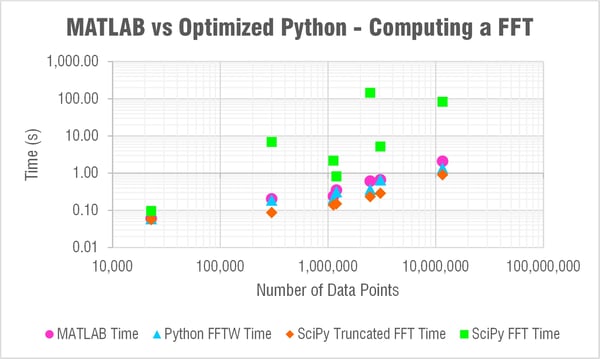
The only trouble with using pyFFTW apparently is the licensing as TheBlackCat nicely explained below in the comments. At enDAQ we've written the Python code for the enDAQ Lab Software (formerly Slam Stick Lab analysis software) all in NumPy due to licensing concerns. But after this testing we've begun looking into a way to obtain a commercial license. As you can see in the results above, pyFFTW is far superior to NumPy's or SciPy's FFT functions and let's you truly compete with MATLAB on performance.
The Code
|
001
002
003
004
005
006
007
008
009
010
011
012
013
014
015
016
017
018
019
020
021
022
023
024
025
026
027
028
029
030
031
032
033
034
035
036
037
038
039
040
041
042
043
044
045
046
047
048
049
050
051
052
053
054
055
056
057
058
059
060
061
062
063
064
065
066
067
068
069
070
071
072
073
074
075
076
077
078
079
080
081
082
083
084
085
086
087
088
089
090
091
092
093
094
095
096
097
098
099
100
101
102
103
104
105
106
107
108
109
110
111
112
113
114
115
116
117
118
119
120
121
122
123
124
125
126
127
128
129
130
131
132
133
134
135
136
137
138
139
140
141
142
143
144
145
146
147
148
149
150
151
152
153
154
155
156
157
158
159
160
161
162
163
164
165
166
167
168
169
170
171
172
173
174
175
176
177
178
179
180
181
182
183
184
185
186
187
188
189
190
191
192
193
|
import matplotlib.pyplot as pltimport pandas as pdimport numpy as npimport tkinter as tkfrom tkinter import filedialogimport timeimport pyfftwimport os###### Functions for testing various FFT methods#####def fftw_builder_test(input_data): pyfftw.forget_wisdom() # This is just here to keep the tests honest, normally pyfftw will remember setup parameters and go more quickly when it is run a second time a = np.array(input_data, dtype='float32') # This turns the input list into a numpy array. We can make it a 32 bit float because the data is all real, no imaginary component fft_obj = pyfftw.builders.rfft(a) # This creates an object which generates the FFT return fft_obj() # And calling the object returns the FFTdef fftw_fast_builder_test(input_data): # See fftw_builder_test for comments pyfftw.forget_wisdom() a = np.array(input_data, dtype='float32') fft_obj = pyfftw.builders.rfft(a, planner_effort='FFTW_ESTIMATE') # FFTW_ESTIMATE is a lower effort planner than the default. This seems to work more quickly for over 8000 points return fft_obj()def fftw_test(input_data): pyfftw.forget_wisdom() # This is just here to keep the tests honest outLength = len(input_data)//2 + 1 # For a real FFT, the output is symetrical. fftw returns only half the data in this case a = pyfftw.empty_aligned(len(input_data), dtype='float32') # This is the input array. It will be cleared when the fft object is created outData = pyfftw.empty_aligned(outLength, dtype='complex64') # This is the output array. Not that the size and type must be appropriate fft_obj = pyfftw.FFTW(a, outData, flags=('FFTW_ESTIMATE',),planning_timelimit=1.0) # NB: The flags tuple has a comma a[:] = np.array(input_data, dtype='float32') # We have to fill the array after fft_obj is created. NB: 'a[:] =' puts data into the existing array, 'a =' creates a new array return fft_obj() # Calling the object returns the FFT of the data now in a. The result is also in outDatadef fftw_test_complex(input_data): # This is fftw_test but running a complex FFT as opposed to a real input FFT. See fftw_test for comments pyfftw.forget_wisdom() outLengthMod = len(input_data)//2 + 1 # Size of expected return data outLength = len(input_data) # For a complex input FFT, we get more data a = pyfftw.empty_aligned(len(input_data), dtype='complex64') # The FFTW determines the type of FFT by the type of input outData = pyfftw.empty_aligned(outLength, dtype='complex64') fft_obj = pyfftw.FFTW(a, outData, flags=('FFTW_ESTIMATE',),planning_timelimit=1.0) a[:] = np.array(input_data, dtype='complex64') return fft_obj()[0:outLengthMod]def fftw_test_default(input_data): # This is fftw_test with different FFTW options. See fftw_test for comments pyfftw.forget_wisdom() outLength = len(input_data)//2 + 1 a = pyfftw.empty_aligned(len(input_data), dtype='float32') outData = pyfftw.empty_aligned(outLength, dtype='complex64') fft_obj = pyfftw.FFTW(a, outData) a[:] = np.array(input_data, dtype='float32') return fft_obj()def fftw_test_no_limit(input_data): # This is fftw_test with different FFTW options. See fftw_test for comments pyfftw.forget_wisdom() outLength = len(input_data)//2 + 1 a = pyfftw.empty_aligned(len(input_data), dtype='float32') outData = pyfftw.empty_aligned(outLength, dtype='complex64') fft_obj = pyfftw.FFTW(a, outData, flags=('FFTW_ESTIMATE',)) a[:] = np.array(input_data, dtype='float32') return fft_obj()def fftw_test_no_flag(input_data): # This is fftw_test with different FFTW options. See fftw_test for comments pyfftw.forget_wisdom() outLength = len(input_data)//2 + 1 a = pyfftw.empty_aligned(len(input_data), dtype='float32') outData = pyfftw.empty_aligned(outLength, dtype='complex64') fft_obj = pyfftw.FFTW(a, outData,planning_timelimit=1.0) a[:] = np.array(input_data, dtype='float32') return fft_obj()def numpy_test(inputData): return np.fft.rfft(inputData) # Numpy is nice and simple!###### Helper Functions#####def write_csv(csv_file_name, headers, data): # Helper function for writing to the CSV file outString = "" for header in headers: outString += "%s," % (data.get(header, "")) outString += "\n" with open(csv_file_name, 'a') as f: f.write(outString)#Prompt user for file#### RUN TIME OPTION!# Set include_plots to True if you want to actually see the plot outputs. They will all be stored up and displayed# at the end of the testinclude_plots = Trueif include_plots: root = tk.Tk() root.withdraw()file_paths = filedialog.askopenfilenames(filetypes=[("Two Column CSV","*.csv")])out_path = filedialog.asksaveasfilename(defaultextension=".csv")print(file_paths)# CSV Setupoutput_headers = ["File", "File Size", "Number of Points", "FFT Time", "FFT Function", "Load Time", "Plot Time", "RMS Time" ]with open(out_path, 'w+') as f: f.write(",".join(output_headers)+"\n")# Tests to run:# Format { "Name" : Function, etc } Test order is undefined#test_functions = {"FFTW" : fftw_test, "FFTW-Complex" : fftw_test_complex, "FFTW-Builder": fftw_builder_test, "FFTW-Default" : fftw_test_default, "FFTW-NoLimit": fftw_test_no_limit, "FFTW-NoFlag": fftw_test_no_flag}test_functions = {"FFTW" : fftw_test, "Builder": fftw_fast_builder_test}figure_count = 1# Loop through each filefor file_path in file_paths: # output_data holds the test info and results. This is written to the file after the FFT is complete output_data = {"File" : os.path.split(file_path)[-1]} output_data["File Size"] = os.path.getsize(file_path) tic = time.clock() df = pd.read_csv(file_path,delimiter=',',header=None,names=["time","data"]) t = df["time"] x = df["data"] toc = time.clock() output_data["Load Time"] = toc-tic print("Load Time:",toc-tic) N = np.int(np.prod(t.shape))#length of the array # Determine variables Fs = 1/(t[1]-t[0]) #sample rate (Hz) T = 1/Fs; output_data["Number of Points"] = N print("# Samples:",N) # Plot Data if include_plots: plt.figure(figure_count) figure_count += 1 plt.plot(t, x) #x plt.xlabel('Time (seconds)') plt.ylabel('Accel (g)') plt.title(file_path) plt.grid() # Compute RMS and Plot tic = time.clock() w = np.int(np.floor(Fs)) #width of the window for computing RMS steps = np.int_(np.floor(N/w)) #Number of steps for RMS t_RMS = np.zeros((steps,1)) #Create array for RMS time values x_RMS = np.zeros((steps,1)) #Create array for RMS values for i in range (0, steps): t_RMS[i] = np.mean(t[(i*w):((i+1)*w)]) x_RMS[i] = np.sqrt(np.mean(x[(i*w):((i+1)*w)]**2)) if include_plots: plt.figure(figure_count) figure_count += 1 plt.plot(t_RMS, x_RMS) plt.xlabel('Time (seconds)') plt.ylabel('RMS Accel (g)') plt.title('RMS - ' + file_path) plt.grid() toc = time.clock() output_data["RMS Time"] = toc-tic print("RMS Time:",toc-tic) # Compute and Plot FFT # Run through each FFT function in test_functions, and test each one. # File data is not reloaded for func_name in test_functions: output_data["FFT Function"] = func_name tic = time.clock() fftData = test_functions[func_name](x) # Execute the FFT xf = np.linspace(0.0, 1.0/(2.0*T), len(fftData)) if include_plots: plt.figure(figure_count) figure_count += 1 plt.plot(xf, 2.0/N * np.abs(fftData)) #[0:np.int(N/2)] plt.grid() plt.xlabel('Frequency (Hz)') plt.ylabel('Accel (g)') plt.title('FFT (%s) - %s' % (func_name, file_path)) toc = time.clock() output_data["FFT Time"] = toc-tic print("FFT Time:",toc-tic) write_csv(out_path, output_headers, output_data)if include_plots: print("Plotting...") plt.show()print("Done!") |
import matplotlib.pyplot as plt
import pandas as pd
import numpy as np
import tkinter as tk
from tkinter import filedialog
import time
import pyfftw
import os

#####
# Functions for testing various FFT methods
#####


def fftw_builder_test(input_data):
    pyfftw.forget_wisdom()       # This is just here to keep the tests honest, normally pyfftw will remember setup parameters and go more quickly when it is run a second time
    a = np.array(input_data, dtype='float32')   # This turns the input list into a numpy array. We can make it a 32 bit float because the data is all real, no imaginary component
    fft_obj = pyfftw.builders.rfft(a)           # This creates an object which generates the FFT
    return fft_obj()                            # And calling the object returns the FFT


def fftw_fast_builder_test(input_data): # See fftw_builder_test for comments
    pyfftw.forget_wisdom()
    a = np.array(input_data, dtype='float32')
    fft_obj = pyfftw.builders.rfft(a, planner_effort='FFTW_ESTIMATE')   # FFTW_ESTIMATE is a lower effort planner than the default. This seems to work more quickly for over 8000 points
    return fft_obj()

def fftw_test(input_data):
    pyfftw.forget_wisdom()                  # This is just here to keep the tests honest
    outLength = len(input_data)//2 + 1      # For a real FFT, the output is symetrical. fftw returns only half the data in this case
    a = pyfftw.empty_aligned(len(input_data), dtype='float32')      # This is the input array. It will be cleared when the fft object is created
    outData = pyfftw.empty_aligned(outLength, dtype='complex64')    # This is the output array. Not that the size and type must be appropriate
    fft_obj = pyfftw.FFTW(a, outData, flags=('FFTW_ESTIMATE',),planning_timelimit=1.0)  # NB: The flags tuple has a comma
    a[:] = np.array(input_data, dtype='float32')    # We have to fill the array after fft_obj is created. NB: 'a[:] =' puts data into the existing array, 'a =' creates a new array
    return fft_obj()                        # Calling the object returns the FFT of the data now in a. The result is also in outData


def fftw_test_complex(input_data):  # This is fftw_test but running a complex FFT as opposed to a real input FFT. See fftw_test for comments
    pyfftw.forget_wisdom()
    outLengthMod = len(input_data)//2 + 1   # Size of expected return data
    outLength = len(input_data)             # For a complex input FFT, we get more data
    a = pyfftw.empty_aligned(len(input_data), dtype='complex64')    # The FFTW determines the type of FFT by the type of input
    outData = pyfftw.empty_aligned(outLength, dtype='complex64')
    fft_obj = pyfftw.FFTW(a, outData, flags=('FFTW_ESTIMATE',),planning_timelimit=1.0)
    a[:] = np.array(input_data, dtype='complex64')
    return fft_obj()[0:outLengthMod]


def fftw_test_default(input_data):  # This is fftw_test with different FFTW options. See fftw_test for comments
    pyfftw.forget_wisdom()
    outLength = len(input_data)//2 + 1
    a = pyfftw.empty_aligned(len(input_data), dtype='float32')
    outData = pyfftw.empty_aligned(outLength, dtype='complex64')
    fft_obj = pyfftw.FFTW(a, outData)
    a[:] = np.array(input_data, dtype='float32')
    return fft_obj()


def fftw_test_no_limit(input_data): # This is fftw_test with different FFTW options. See fftw_test for comments
    pyfftw.forget_wisdom()
    outLength = len(input_data)//2 + 1
    a = pyfftw.empty_aligned(len(input_data), dtype='float32')
    outData = pyfftw.empty_aligned(outLength, dtype='complex64')
    fft_obj = pyfftw.FFTW(a, outData, flags=('FFTW_ESTIMATE',))
    a[:] = np.array(input_data, dtype='float32')
    return fft_obj()


def fftw_test_no_flag(input_data):      # This is fftw_test with different FFTW options. See fftw_test for comments
    pyfftw.forget_wisdom()
    outLength = len(input_data)//2 + 1
    a = pyfftw.empty_aligned(len(input_data), dtype='float32')
    outData = pyfftw.empty_aligned(outLength, dtype='complex64')
    fft_obj = pyfftw.FFTW(a, outData,planning_timelimit=1.0)
    a[:] = np.array(input_data, dtype='float32')
    return fft_obj()


def numpy_test(inputData):
    return np.fft.rfft(inputData)       # Numpy is nice and simple!


#####
# Helper Functions
#####

def write_csv(csv_file_name, headers, data):        # Helper function for writing to the CSV file
    outString = ""
    for header in headers:
        outString += "%s," % (data.get(header, ""))
    outString += "\n"
    with open(csv_file_name, 'a') as f:
        f.write(outString)


#Prompt user for file
###
# RUN TIME OPTION!
# Set include_plots to True if you want to actually see the plot outputs. They will all be stored up and displayed
# at the end of the test
include_plots = True
if include_plots:
    root = tk.Tk()
    root.withdraw()
file_paths = filedialog.askopenfilenames(filetypes=[("Two Column CSV","*.csv")])
out_path = filedialog.asksaveasfilename(defaultextension=".csv")
print(file_paths)

# CSV Setup
output_headers = ["File", "File Size", "Number of Points", "FFT Time", "FFT Function", "Load Time", "Plot Time", "RMS Time" ]
with open(out_path, 'w+') as f:
    f.write(",".join(output_headers)+"\n")

# Tests to run:
# Format { "Name" : Function, etc } Test order is undefined
#test_functions = {"FFTW" : fftw_test, "FFTW-Complex" : fftw_test_complex, "FFTW-Builder": fftw_builder_test, "FFTW-Default" : fftw_test_default, "FFTW-NoLimit": fftw_test_no_limit, "FFTW-NoFlag": fftw_test_no_flag}
test_functions = {"FFTW" : fftw_test, "Builder": fftw_fast_builder_test}
figure_count = 1
# Loop through each file
for file_path in file_paths:
    # output_data holds the test info and results. This is written to the file after the FFT is complete
    output_data = {"File" : os.path.split(file_path)[-1]}
    output_data["File Size"] = os.path.getsize(file_path)
    tic = time.clock()
    df = pd.read_csv(file_path,delimiter=',',header=None,names=["time","data"])
    t = df["time"]
    x = df["data"]
    toc = time.clock()
    output_data["Load Time"] = toc-tic
    print("Load Time:",toc-tic)

    N = np.int(np.prod(t.shape))#length of the array
    # Determine variables
    Fs = 1/(t[1]-t[0])  #sample rate (Hz)
    T = 1/Fs;
    output_data["Number of Points"] = N
    print("# Samples:",N)

    # Plot Data
    if include_plots:
        plt.figure(figure_count)
        figure_count += 1
        plt.plot(t, x)  #x
        plt.xlabel('Time (seconds)')
        plt.ylabel('Accel (g)')
        plt.title(file_path)
        plt.grid()

    # Compute RMS and Plot
    tic = time.clock()
    w = np.int(np.floor(Fs))         #width of the window for computing RMS
    steps = np.int_(np.floor(N/w))   #Number of steps for RMS
    t_RMS = np.zeros((steps,1))      #Create array for RMS time values
    x_RMS = np.zeros((steps,1))      #Create array for RMS values
    for i in range (0, steps):
        t_RMS[i] = np.mean(t[(i*w):((i+1)*w)])
        x_RMS[i] = np.sqrt(np.mean(x[(i*w):((i+1)*w)]**2))
    if include_plots:
        plt.figure(figure_count)
        figure_count += 1
        plt.plot(t_RMS, x_RMS)
        plt.xlabel('Time (seconds)')
        plt.ylabel('RMS Accel (g)')
        plt.title('RMS - ' + file_path)
        plt.grid()
    toc = time.clock()
    output_data["RMS Time"] = toc-tic
    print("RMS Time:",toc-tic)

    # Compute and Plot FFT
    # Run through each FFT function in test_functions, and test each one.
    # File data is not reloaded
    for func_name in test_functions:
        output_data["FFT Function"] = func_name
        tic = time.clock()
        fftData = test_functions[func_name](x)          # Execute the FFT
        xf = np.linspace(0.0, 1.0/(2.0*T), len(fftData))
        if include_plots:
            plt.figure(figure_count)
            figure_count += 1
            plt.plot(xf, 2.0/N * np.abs(fftData))       #[0:np.int(N/2)]
            plt.grid()
            plt.xlabel('Frequency (Hz)')
            plt.ylabel('Accel (g)')
            plt.title('FFT (%s) - %s' % (func_name, file_path))
        toc = time.clock()
        output_data["FFT Time"] = toc-tic
        print("FFT Time:",toc-tic)
        write_csv(out_path, output_headers, output_data)
if include_plots:
    print("Plotting...")
    plt.show()
print("Done!")
Conclusions
A couple major take-aways:
- Python is an impressive free alternative to MATLAB
- Python's SciPy FFT function is inferior to MATLAB's, especially when dealing with data sets that have a length not equal to a power of 2
- Forget about even trying to compute a FFT on an array that has a length equal to a prime number in SciPy or Numpy
- Best practice in SciPy or NumPy is to truncate the array to the last power of 2
- pyFFTW is far superior to SciPy's or NumPy's FFT function and offers comparable performance to MATLAB
- The only downside is the licensing issue if you are distributing any software
- The pandas library is a must have for Python users loading CSV files
I originally concluded that MATLAB has better built in functions compared to Python. But the truth is that Python has those same functions and computing abilities! The only trouble is that you have to go digging a bit to find them and compile it all together. And the extra bit of work is a hurdle for a user like me: someone with a lot of MATLAB experience and a company paying for my commercial license.
This testing completely opened my eyes to the possibilities of Python though. It’s intriguing to have a truly free alternative to MATLAB and one that can get you the same analysis results. For folks that are turned off by the high price of MATLAB then Python is a great option. If cost is not a concern and you’re mostly interested in technical analysis of matrices, then MATLAB may be a little easier to work with. But if you are going to be doing any programming besides technical analysis, Python seems to be the far better option.
I’m curious to see what you think though, do you prefer MATLAB or Python? Select your opinion below. I also encourage you to download the data to try the testing for yourself! And if you'd like to do more with Python for vibration data analysis, check out our post Top 12 Vibration Metrics to Monitor & How to Calculate Them which provides source code on how all of these calculations were done in Python.
For an introduction to Python, check out our article Get Started with Python: Why and How Mechanical Engineers Should Make the Switch.