That is the fundamental question in digital data acquisition.
In this blog I will get started on the answer to this question; but as you'll see - it's not easy! I'll go through two examples: one using a sine wave and the second using real data (download) I recorded from a pyrotechnic pin puller to show how it would be corrupted by improper sampling. Hopefully by the end of this discussion you'll have a better understand of aliasing.
In this edition, we will discuss what causes aliasing. Join us for follow-on blogs to see what you can do to minimize the resulting errors.
A Goldilocks Dilemma
In the data acquisition world, we describe the sampling parameter in terms of points per cycle. It is easy to understand when we are measuring a sine wave.
Let’s see if we can make it a Goldilocks decision: What is too fast, too slow, or just right?
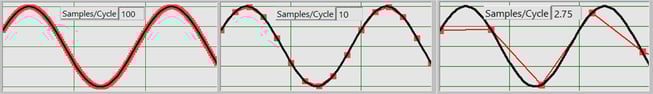
The first frame in Figure 1 shows 100, the second 10, and the third, 2.75 points/cycle.
- Obviously, 100 points/cycle defines the sine wave really well.
- 10 points/cycle looks pretty good but, if we are interested in peak values, and we are unlucky enough to have the points equidistant from the peak, we have an error of ~5%. Is this OK?
- At 2.75 points/cycle, it looks like we are in real trouble.
But it’s not that simple. As it turns out, it’s not a really Goldilocks dilemma... all of the above are just right... depending on your requirements and available tools. We need to delve further.
Shannon's Theorem
In 1948 Claude Shannon published a paper that contained the fundamental law for discrete time history sampling. A paraphrase of what is now called Shannon’s Theorem is:
If we acquire more than two points/cycle
of the highest frequency in the signal
the waveform is completely defined.
It is pretty straightforward:
- If we sample at more than twice the highest frequency in the signal we satisfy Shannon’s Theorem. All of the examples satisfy this criterion.
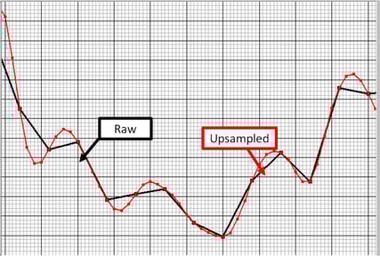
- If we satisfy Shannon's Theorem, we know everything there is to know about the signal. This means that, if we have the appropriate tools (“Resampling”, or “Upsampling”), we can reconstruct any time history to any resolution that we want (Figure 2). So, 2.75 (or any number greater that 2) is OK. We will discuss this magic trick in a later blog.
But, it’s not so simple..the phrase: “of the highest frequency component in the signal” is the problem.
We know that all real signals have an infinite bandwidth (there are frequency components out to light frequency, and beyond…They may be small but they are there).
So..Shannon’s Theorem is ALWAYS VIOLATED!!
So, we should pack our bags and go home. Digital data acquisition does not work!
But, we know it does work… (Steve Hanly told us so). So what’s going on?
Aliasing
Violation of Shannon’s Theorem produces errors. These errors are called Aliasing. The errors can be small or large depending on how the data is acquired. The challenge, and our objective, is to assure that they are very small.
Nyquist Frequency
The term aliasing is a misnomer but the result is that any energy that is above ½ of the sample rate (called the Nyquist Frequency (Fn)) appears at the wrong frequency. Any signal components above Fn are “aliased” to lower frequencies where they are superimposed on the truth. This is obviously an error.
Aliasing Demonstration Video
The aliasing phenomenon is much more easily seen (and understood) in the frequency, or spectral, domain. To do this, we use the Fourier Transform to calculate the spectrum. Once we have that tool we can do a demo. To keep it simple we will use a sine wave input. The spectrum of a sine wave is a single “spike” in the spectrum. Figure 3 provides an overview of aliasing by "Captain Alias."
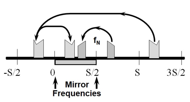
Frequency Folding
What should be obvious from the movie is that any frequency components above the Nyquist frequency will corrupt the signal that we are interested in. They will fold, and refold, until they wind up in the range we care about (Figure 4).
Real Shock Data
Of course, real life is normally not as simple as a sine wave.
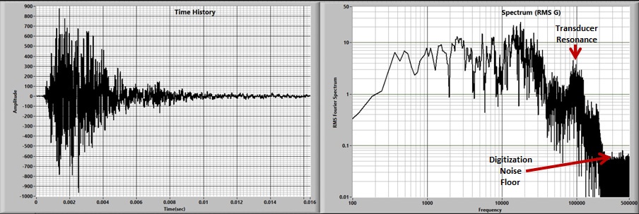
The time history and spectrum of the pyroshock test that I use so often (that is available to download) are shown in Figure 5.
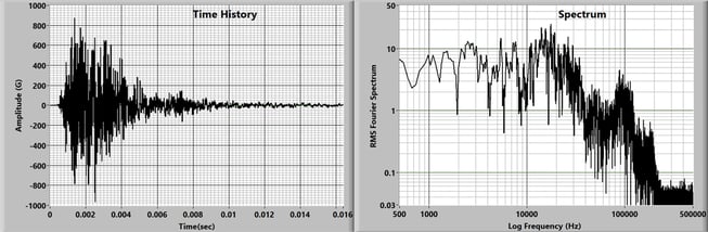
Again, the real clue to what is going on is in the spectrum. The critical feature is that the magnitude of the spectrum is small (reduced to the digitization noise floor) above ~250KHz. Is this data set aliased? Yes!! All real data sets are aliased to some extent. However, the fact that that the level is very small (compared to the main signal) near the Nyquist frequency implies that there is not much energy at higher frequencies so that the errors are small. In fact, since the spectrum is reduced to the digitization level, the resulting errors are as small as we can make them with this data acquisition system.
Now, let’s reduce the sample rate by decimating the time history (i.e. keep 1 out of every N points). We will do a fairly extreme example to make it obvious what is going on. The boss tells us that only frequencies up to 10 KHz are of interest so we will take the knowledge we have and sample at 25,000 samples per second giving us 2.5 points/cycle at the highest frequency of interest. The result is in Figure 6.
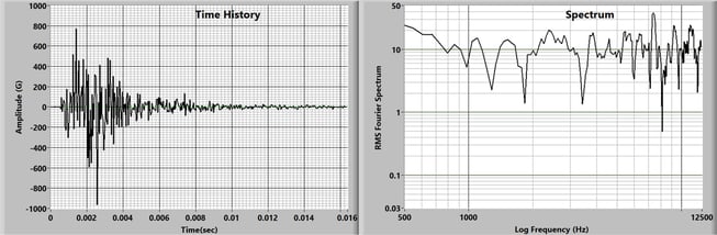
Inspection shows:
- The time history looks pretty reasonable.. There is no evidence in it that there is a problem.
- However, when we look at the spectrum, it is not reduced to insignificant levels at the Nyquist frequency. The implication (which is correct) is that there is significant energy at higher frequency. This “litmus test” indicated that the data is probably badly corrupted by aliasing. However, from this record, there is no way to tell how bad the corruption is.
Figure 7 shows the overlay of the truth (black) over the undersampled (red) results. The time histories are pretty much alike. In the undersampled data, lots of the peaks are missed because only 1 point in 40 of the original signal has been recorded. However, the RMS levels of both recordings are essentially the same.
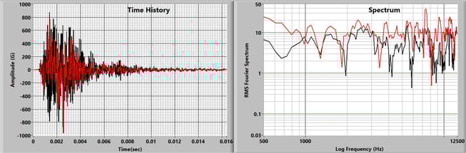
The spectrum plots show the problem: The undersampled spectrum (red) is significantly higher than the truth (black) at almost all frequencies. This is the result of the frequency components above the Nyquist frequency being folded into (and added to) the true result. (Comment: If the spectrum is wrong, so is the time history!)
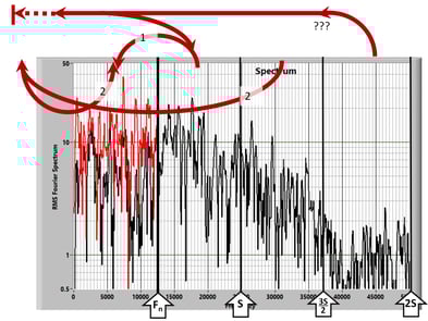
- Energy between the Nyquist frequency and the sample rate is superimposed on the correct result below Fn.
- Energy between the sample rate and 1.5S is folded around Fn to below zero. It is then refolded around zero into the range of interest.
- All energy above Fn is added to the correct data via multiple folding.
So, we are in real trouble. Although the aliasing problem for this signal can be solved by sampling at over 500,000 samples/second, this is not always an available option.
Those in the aerospace shock industry may recognize this phenomenon as the root cause of one of the worst (and most expensive) testing errors in history. A large number of spacecraft qualification tests were incorrectly accepted because the indicated spectral response was higher than the truth. This resulted in the false-positive passing of the test’s specification.
Once the Data Set is Acquired, any Aliasing Errors are Included in the Measured Time History.
- There is no way to tell how large the errors are.
- No amount of data manipulation will fix it. The data set in Figure 6 is irretrievably corrupt.
- Alias errors are only minimized by proper setup of the data acquisition before the test.
Whoops… Did We Get Sidetracked?
Did we answer the original question: How fast must we sample? Not yet. To put it simply, it’s simply not that simple. There is a lot more to it.
The next blog entry will explore the options and tradeoffs involved in making this measurement with lower sample rates by using analog or hybrid analog/digital low-pass (anti-alias) filters. We will be faced with another Goldilocks decision: Bessel, Butterworth, Elliptical, or Sigma-Delta. Which one will she choose?
Send a Comment or Question to Strether

One of the reasons I've been writing these blogs is to get a discussion going. Please reach out privately to me with any questions or comments you may have.
You can participate by:
- Entering comments/questions below in the Comments Section at the end of the blog. This will obviously be public to all readers.
- Contact me directly. I will respond privately and (hopefully) promptly. If appropriate, your question could be the subject of a future blog.
This blog is meant to be a seminar... not a lecture. I need your help & feedback to make it good!
Disclaimer
Strether has no official connection to Mide or enDAQ, a division of Mide, and does not endorse Mide’s, or any other vendor’s, product unless it is expressly discussed in his blog posts.
Additional Resources
If you'd like to learn a little more about various aspects in shock and vibration testing and analysis, download our free Shock & Vibration Testing Overview eBook. In there are some examples, background, and a ton of links to where you can learn more. And as always, don't hesitate to reach out to us if you have any questions!
Download Strether's PyroShock Time History File
File Details
- Piezoelectric Shock Accelerometer mounted next to a pyrotechnic pin puller.
- Sample rate: 106 Samples/Second
- Data “Cleanup”: 2-Pole Butterworth at 100 Hz.