The goal in condition monitoring is to detect an incipient defect and predict when failure will occur. But the process of predicting a failure isn't always straightforward.

In this post I'll provide an overview of condition monitoring of bearings along with some theory about bearings themselves. Then I'll provide a couple examples where I perform an envelope analysis and compare the results to a digital implementation similar to the PeakVue method which for the purposes of this article I will call the digital PeakVue method. The post provides many external references to hopefully be of some help to you as you look to perform your own condition monitoring of bearings!

Condition Monitoring Overview

Condition monitoring and predicting a potential failure will allow the defective part to be replaced during a scheduled maintenance shutdown prior to failure.  For a detailed review of predictive maintenance, there are many sources available such as this from Azima. 

The best strategy for critical machinery, for which unscheduled downtime results in significant costs, is an online predictive maintenance system.  There are many such systems, with brands like CSI, SKF and GE Bentley Nevada being popular.  One of the most advanced systems for gear trains with anti-friction bearings is offered by Tensor Systems.

Vibration is typically measured with accelerometers, unless hydrodynamic bearings are monitored, in which case proximity (displacement) probes are used.  When data is collected with accelerometers, it is usually displayed as velocity, since machine (and human) damage is most closely represented by velocity (as compared to displacement or acceleration) with the least dependence on frequency.

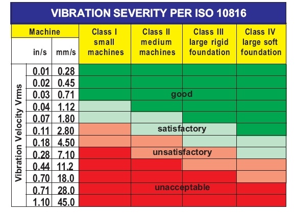
Typically when vibration amplitude exceeds a certain level, such as that given in Figure 1, there is a problem on the machine.  Often the problem can be determined by the signature (spectrum) of the vibration.  Ideally, this signature includes phase as well as amplitude.

Incipient defects in bearings will not generally show up in this type of analysis, however, as the amplitudes are much too small.

Types of Bearings

Hydrodynamic Bearings

There are two broad bearing types used in modern machinery.  One is the hydrodynamic bearing, also known as a fluid film bearing.  These are typically used on larger industrial machinery.  Motors transition to fluid film bearing at around the 5000 HP range.  Hydrodynamic bearings are also the bearings of choice for your car engine.  Your crankshaft main bearings, connecting rod bearings, and camshaft bearings are all fluid film bearings. 

For large industrial machines, the earliest company that did a lot of research into predictive maintenance was Bentley Nevada, now owned by GE.  They invented the proximity probe that is normally used to measure the vibration of these bearings, the diagnostic techniques, and the monitoring system.  Often when a trip occurs, causing the machine to shut down, the time histories from the proximity probes are collected along with a 1 pulse per revolution (PPR) signal of the rotational speed.  These signals can then be analyzed to help determine the cause of the trip.

It is not the intent of this blog to focus on hydrodynamic bearings. 

Anti-Friction Bearings

The second main class of bearings is referred to as anti-friction bearings, which include ball bearings and roller bearings.  Each of these bearings has 4 fault frequencies:

• Fundamental Train Frequency (FTF)
• Ball Pass Frequency on the Inner race (BPFI)
• Ball Pass Frequency on the Outer race (BPFO)
• Ball Spin Frequency (BSF). 

The equations to determine the frequencies can be found by an internet search for bearing frequencies. This website provides both the equations and a table of bearings showing the defect orders.  Order is a convenient term for the number of occurrences of a vibration during 1 shaft rotation.  For machines that are absolutely constant in speed, order is calculated by dividing the frequency by the shaft rotational speed.  Since no shaft is absolutely constant in speed this method can cause smearing of spectral peaks, especially at higher frequencies.  This can be prevented with resampling the time domain data into the angle domain, normally performed by using a tachometer to continuously measure the shaft rotational speed.

There are two additional factors that affect the bearing frequencies.  As the loading on the bearing changes, the pitch angle can change, resulting in a slightly different frequency.  Additionally, all bearings will have some clearance.  When the ball (roller) is in the load zone, the forces constraining it to move deterministically are great.  However, when the ball is in the no load zone, these forces are minimal, and a minor amount of slip will occur.  This slip will result in actual bearing frequencies slightly different from those predicted by the equations.

It might seem pretty straightforward to use spectrum analysis to determine whether one of these frequencies is present.  However, the impact forces when a crack is initiated are small, and thus the resulting bearing vibration is dwarfed by all the other vibration. 

Stresses in Anti-Friction Bearings

Back in the late 1800’s Hertz developed the equations to predict stress levels in curved elastic solids in contact with each other (more information available on Wikipedia).  Bearing and gear manufacturers quickly picked up on this to aid in the design of their respective products.  This analysis shows maximum stress levels are slightly below the surface, in particular, any discontinuity in the bearing steel at the maximum stress region could be the location of crack initiation.  With the advent of electric arc smelting furnaces, the number of impurities in bearing steels has been greatly reduced, and bearing life has increased.

Cracks that form below the surface of the metal will migrate to the surface with use.  Once a crack is at the surface of the race, it will be impacted by the balls as they pass over the crack.  Because this impact is metal on metal, and the crack is tiny, it is a very short impact, with a reasonably high peak force but a limited impulse (the area under the force time curve).  This is a good representation of the Dirac-delta function. 

Those that know the selection process of modal hammer tips will recognize that this impact in the frequency domain has a very low excitation level, but the force extends to very high frequencies  In practice, it has been found to extend well into the kHz range. 

Since the bearing defect forces are so low and are mingled with many other excitations, it is difficult to see in the vibration at these low frequencies.  However since the force extends into the high-frequency range it excites bearing resonant frequencies and acts as an amplitude modulation component on these frequencies.

Anti-Friction Failure Criteria

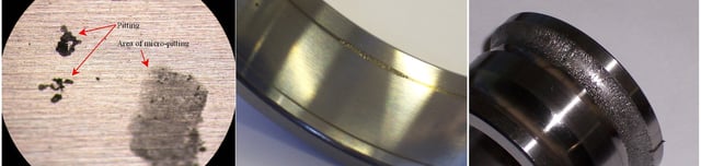
Anti-friction bearings have a number of failure stages.  The first stage is normal operation.  The next stage of failure is a small crack or some other minor defect which will excite a resonance in the bearing.  A bearing can run a long time with minor defects.  Often these defects can only be detected with envelope analysis or similar techniques. 

Over time however, the metal near the crack starts spalling.  When this happens the bearing operation becomes much rougher, with more vibrational energy and the defect frequencies become noticeable. 

The final stage is when the complete raceway becomes spalled.  The discrete bearing frequencies tend to disappear and random broad band vibration is noticed.  These stages are shown below in Figure 2.

Amplitude Demodulation

Normal spectrum analysis has difficulty showing the initial stages of bearing failure as there is very little energy in the signal.  The bearing vibration is often not detectable due to the presence of process noise. 

To extract this signal, amplitude demodulation techniques have been developed.  This term is synominous with envelope analysis, as the envelope of a signal is the amplitude of the carrier frequency.  There are a variety of algorithms to perform this task, with the algorithm of choice changing with the evolution of computer processing power, and whether the demodulation needs to be performed in real time or if it can be done as a post-processing operation.  The currently recommended algorithm for bearing diagnostics is given in the book, “Vibration Based Condition Monitoring” by Robert Randall.  

A similar technique is called PeakVue, patented by CSI, with the patent filing date slightly over 20 years ago, meaning the patent has now expired.  

Separating Bearing Frequencies from Gear Mesh Frequencies

Normally the highest vibration levels from gear trains are at a harmonic of a shaft rotational speed.  Unbalance occurs at the shaft rotational speed, misalignment at both shaft rotational speed and two times this speed.  Gear mesh frequency is also at a harmonic of shaft rotational speed.  If the device being driven is a pump or fan, there will be a blade or vane pass frequency, which again is a harmonic of the shaft rotational speed.  However, if we look at the bearing frequencies shown in the earlier reference, the table shows there are very few bearings having a bearing defect frequency which is exactly an integer multiple of the shaft rotational frequency.  Even then we must remember that there will likely be a little slip so the probability of a bearing frequency being precisely an integer multiple of shaft speed is nil, if we can do an accurate enough spectral analysis.  The Tensor Systems uses this knowledge to separate bearing defects from gear mesh and other shaft related defects.  A tachometer obtains the shaft rotational speed, and the vibration signal is resampled into the angle/order domain.  The end result is a much more automated system to determine where faults lie.

However, since the vibration at the bearing fault frequencies in the initial stages of a bearing fault is so low a more robust approach is required to determine this stage of the fault.  After the advent of the FFT algorithm, smart people realized that bearing resonant frequencies in the kHz range were excited by bearing faults, and the overall vibration level at these frequencies was measured.  With additional research, it was found that the vibration signal could be amplitude demodulated to obtain the bearing impacts and then the demodulated signal could be transformed to the frequency domain to detect the bearing frequencies.

Envelope and Digital PeakVue Example

I coded the envelope analysis algorithm recommended above using Matlab.  In addition, I coded an algorithm similar to PeakVue to compare with envelope analysis.  Sample defective bearing data from Case Western University was used for the first algorithm comparison case. 

The data is from the 12k Fan End Bearing Fault Data with 0.007” fault diameter and with the fault being on the inner race with a 3HP motor load.  The data analyzed here are from the faulty fan end bearing. 

A portion of the time history of this bearing failure is shown in Figure 3.

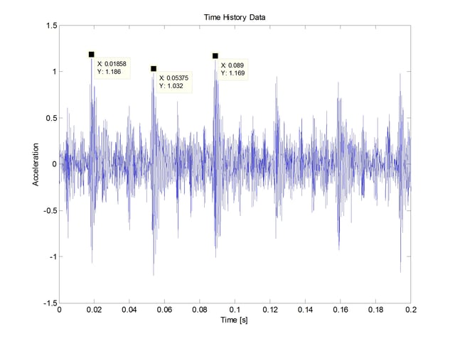
The dominant characteristic is the occurrence of impacts.  The difference in time between impacts shows that they are occurring at shaft rotational speed.  A balance problem would show a sinusoidal vibration, not evident in this figure.  From this data, I suspect this may be an alignment issue.  As an aside, it should be possible to obtain extremely precise rotational speed and phase angle data using a phase demodulation technique.  But that would require another blog.

Performing a spectral analysis on this data gives the following information in Figure 4.

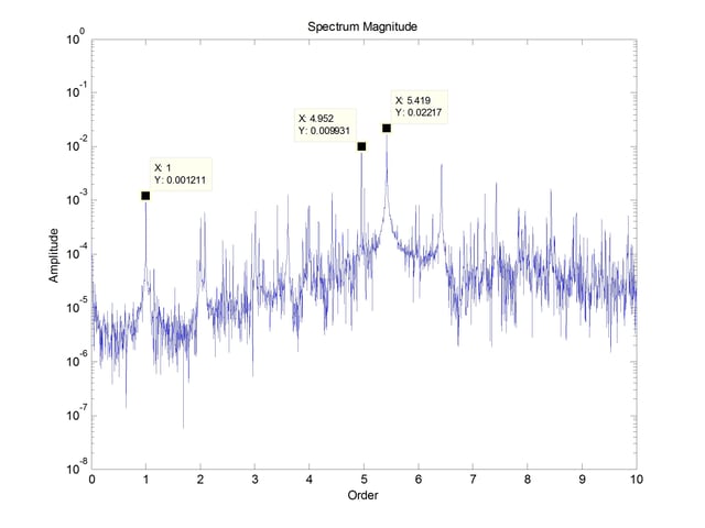
Note that the abscissa has been plotted as orders.  The conversion to orders was done by dividing the frequency by the recorded shaft rotational speed and then tweaked to ensure that the first harmonic is exactly 1.  A true order plot would have had the rotational speed recorded with the vibration and had the vibration data resampled into the angle domain.  Figure 4 shows harmonics of the rotational speed, the inner race frequency of both the drive end (DE) and fan end (FE) bearings and some difference frequencies.  According to Case Western only the FE bearing has a fault, so this spectrum is not helpful in determining the fault.

Envelope analysis is used to obtain reliable bearing defect information from bearing resonances in the high-frequency portion of the spectrum.  The first step in performing the envelope analysis is to transform the complete time history into the frequency domain.  Current FFT algorithms such as FFTW provided with Matlab are efficient even when the number of data points is not a power of 2.  The spectrum of this time history is shown in Figure 5.

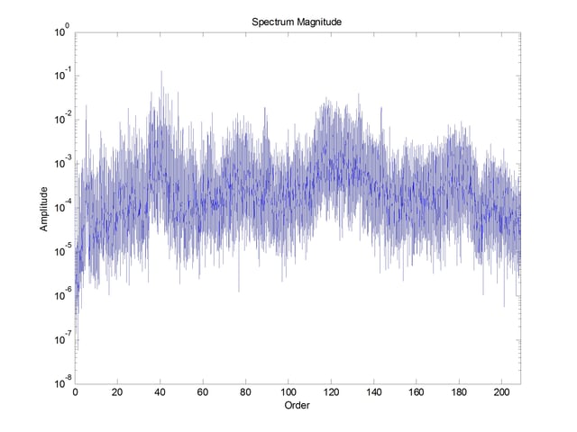
From this spectrum, the region for amplitude demodulation is selected around an existing resonance.  Resonance is determined by the eyeball average amplitude of the signal.  In this case, the data from 109 – 146 orders was selected. 

The selected data is moved to the left in the frequency domain.  At least as many zeros as there is data is appended to the right of this data, depending upon the number of time points desired.  The data is inverse transformed back to the time domain.  The amplitude of the complex time domain is the amplitude of the modulated signal.  This data is then transformed back to the frequency domain to give the spectrum of the amplitude modulated signal.

The resulting spectrum from the demodulated data is shown in Figure 6.

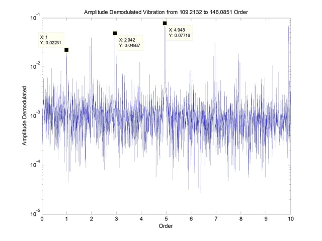
This spectrum shows both the rotational speed and the inner race defect frequency, with the defect frequency being the highest peak in the spectrum.  Also present are running speed sidebands within this spectrum.

To complement this analysis, the digital PeakVue analysis was carried out.  The dataset was high pass filtered at 109 orders.  This filtered data was then analyzed for the maximum value within each block of data, with spectrum analysis performed on these maximum values.  The resulting spectrum is shown in Figure 7.

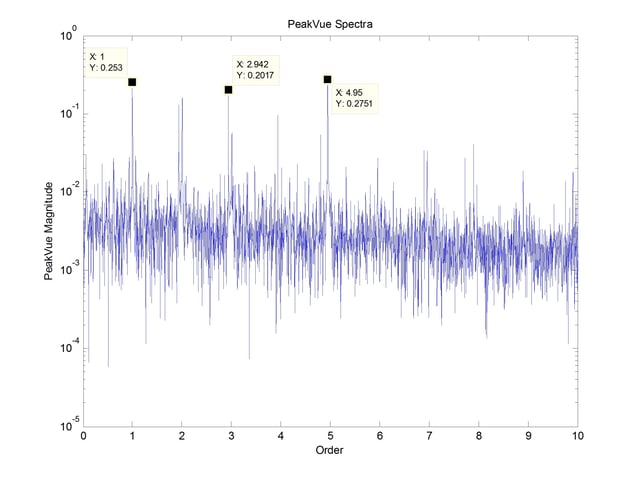
The results from this analysis, very similar to the results of the envelope analysis, indicate that both algorithms perform equally well.  Since the defect frequency also shows up quite strongly in the baseband spectrum, I suspect this simulated fault is not typical of most early stage bearing faults.

Since this is a blog on the Mide website, it would not be complete without using data acquired with one of their accelerometers.  I mounted an enDAQ sensor on an old shop grinder that exhibits an annoying harsh sound.  I always wondered if it had a bad bearing, but it has not received enough use to worry about. 

The spectrum of the vibration of this grinder is shown below in Figure 8.

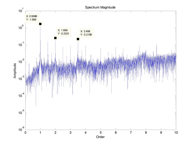
A strobe light was used to determine the rotational frequency of 59.48 Hz.  The spectrum shows that the dominant vibration occurs at rotational speed with the second harmonic amplitude being almost an order of magnitude lower.  Also present are half harmonics.  Both the harmonics and half harmonics are indicative of looseness likely excessive clearance in the bearings.

The spectrum of the envelope analysis is shown in Figure 9.

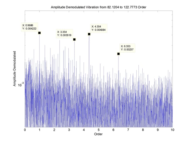
Present is the rotational speed again but also 4.35 order along with running speed sidebands.  Since the bearing type is not known, it cannot be matched to a bearing frequency, but it is certainly plausible that this is caused by a defect on a race of the bearing.  It is also possible that the bearing is so worn, that its frequency is still present but the wear is contributing to the looseness suspected from the previous spectrum.

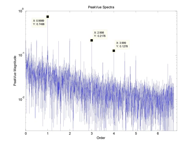
An analysis similar to PeakVue is shown below in Figure 10, This spectrum shows the harmonics and half harmonics of the running speed, but does not show any potential bearing defect, as the envelope analysis did.

Conclusions

In comparing the envelope analysis with the digital PeakVue method, with just the two tests, the envelope technique seems more robust.  When post processing data, the envelope analysis technique is easier to perform.  However, the digital PeakVue method is more straightforward for real time processing. 

An ideal implementation for on-line analysis is to resample the data into the order domain using a tachometer, as done by Tensor Systems. 

For more on this topic, visit our dedicated Wireless Vibration Monitoring Systems resource page. There you’ll find more blog posts, case studies, webinars, software, and products focused on your condition monitoring and maintenance needs.

About the Author

Jake Zwart specializes in vibration analysis to add value to companies, assisting them in providing a more uniform product and reducing failures.  Initially Jake only used commercial software but his interest in the underlying concepts and shortcomings of commercial systems nudged him into developing additional algorithms. Jake has no ties to any company mentioned in this blog post except for Tensor Systems. More information is available at www.spectrum-tec.com  or contact him directly at jake.zwart@spectrum-tec.com