The Best of all Possible Worlds?
In previous blogs, we discussed the need for alias protection in the digital data acquisition process and the options that we have to provide it. We showed that different low-pass-filter strategies produced significantly different results and that the some of the options were more “efficient” (i.e. allowed lower sample rates than others). In the last entry, we discussed how the analog filter options: Bessel, Butterworth, and elliptical, are designed. Here, we will discuss the hybrid (analog/digital) option that, for many applications, provides huge advantages over their analog siblings.
This section relies heavily on concepts and terminology discussed in earlier blogs. Please take a look at them if you haven't already.
Overview
The objective is to provide a digitizer that does most of its work in the digital domain. Why:
- Digital calculations are absolutely repeatable.
- We can make a "better" filter there.
- It is a whole lot cheaper.
However, we can’t do it all in the digital domain. The aliasing issue, discussed at great length in the previous blogs, must be faced (and solved) in the analog domain. Our objective here is to minimize the analog contribution by using very simple filters. One- or two-pole filters are more stable, induce less distortion, and are obviously cheaper than the multi-pole/multi-zero analog filters discussed in the earlier blogs.
This discussion is divided into three major sections:
- The basic concept of the oversampling process and a specific implementation.
- A discussion of the delta-sigma modulation process that is used for the digitization process in most oversampling systems.
- A brief description of the Finite Impulse Response (FIR) filter concept that gives oversampling data acquisition systems near-perfect characteristics.
The Hybrid Analog/Digital “Oversampling” Digitizer
First we have to solve the alias-error issue. From previous discussions, we know that aliasing will occur if there is an unacceptable amount of energy that will fold around the Nyquist Frequency (= Sample Rate/2) into our frequency range of interest.
The first stage (analog) of the hybrid process shown in Figure 1.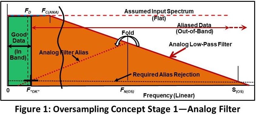
The objective is to assure that data within in our Desired Bandwidth (zero frequency to FD) is adequately alias protected and that it is not significantly distorted.
As we did in earlier examples, we will assume that the input energy has a spectrum that is constant over all frequencies (dashed red line--); an assumption that is normally, but not always, conservative.
Next, we apply an analog filter with a cutoff frequency of FC(ANA). This frequency must be significantly above FD to assure that there is acceptably small distortion (amplitude modification and phase nonlinearity) within that range.
We then sample the data at a high sample rate S(OS). We select a sample rate that assures that the aliasing error is attenuated to the required level (“Required Aliasing Rejection”) at F”OK” (which also must be significantly above FD).
What we have now is:
- Alias protected data from zero frequency to F”OK” (Green). We can do any digital manipulation we want to within that frequency range.
- A huge amount of out of band-energy (that is also corrupted by aliasing) above F”OK” (Orange).
Next, we will zoom into the frequency range we care about and do the digital operations (Figure 2).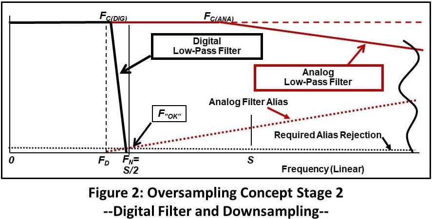
A very-sharp digital filter is applied with a cutoff FC(DIG) slightly above FD. The cutoff characteristic provides an attenuation of at least “Required Alias Rejection” at F”OK”. This rejects the out-of-band energy.
Last, we reduce the sample rate S so that Nyquist Frequency FN is ~= FOK. The result is alias-protected data to F”OK (which is above FD) with a sample rate that is appropriate for our application.
The ratio of the reduction in sample rate (S(OS)/S) is called the Oversampling Ratio (R). For practical reasons, to be shown later, it must be an integer. Although any ratio can be used, common values are 16 and 32.
Implementing an Oversampling System
The following example shows how we might design an oversampling system. The objective to acquire data with a 10KHz desired frequency range (0 to FD) with near-perfect alias rejection and minimal distortion.
Figure 3 shows the analog/oversampling stage:
- Use a 2-pole analog Butterworth filter at 31 KHz (FC).
- Sample at 1 million samples/second (S(OS)).
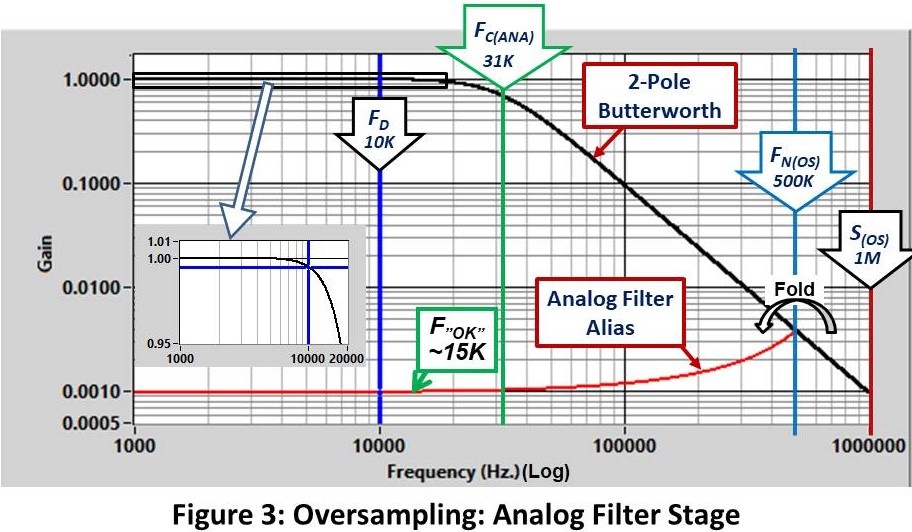
This results in an alias rejection of > 1000/1 at ~15KHz. (F”OK”) and an amplitude error of <0.5% from zero frequency to FD. (Inset Plot).
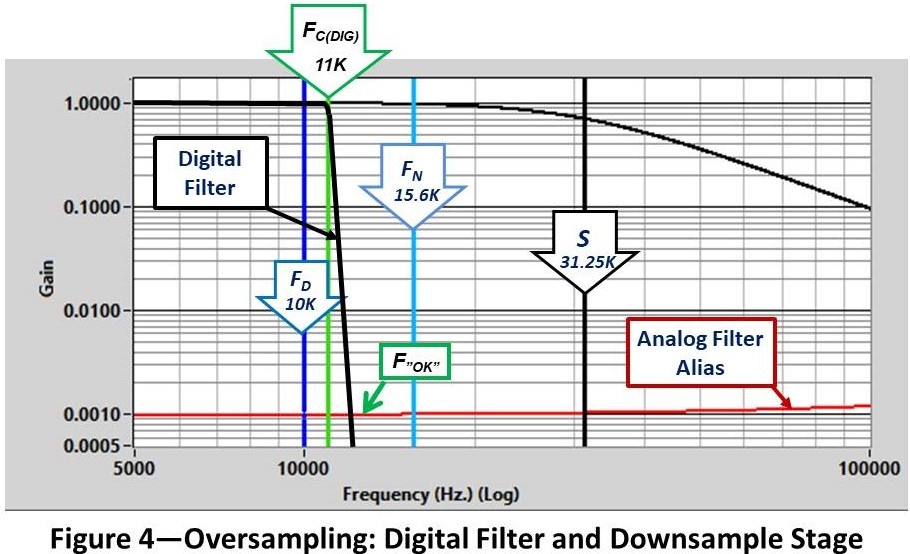
Next, we will apply a digital filter and down-sample the result (Figure 4).
- Digital filter to 11 KHz. (FC(DIG)) using a very-sharp, linear-phase, filter (to be discussed shortly). The filter reduces the spectrum to “Required Alias Rejection” at F”OK”
- Decimate (“Downsample”) by 32 (R) to 31.25K S/S (S).. This gives 3.125 points/cycle at 10 KHz.
As discussed in the 3rd blog, one of the advantages of the oversampling/sigma-delta approach is that relatively low sample ratios (points/cycle at FD) can be used. When we are doing spectral analysis, this is not a problem. However, for time domain applications, more points/cycle may be required. This can be provided by up-sampling in post processing, to be discussed in a later blog.
More Bad Terminology
The word Decimate looks like it has something to do with 10 (and it did in the classical meaning). However, in our case, it means to keep one out of every N data points in our time history. So, if I was decimating by 8, I would keep the 1st, 9th, 17th… points. This results in a reduction of the sample rate by 8.
It’s as simple as that, but.. Where are we going to get a good 16 (or more) bit analog-to-digital converter that samples at a million samples/second? (Actually, it’s not that hard now but 25 years ago it was a real challenge.) And, for lots of applications, we need a higher FD which, of course, requires a higher sample rate S(OS)).
…then.. Along Came Sigma Delta!
The concept of Delta Sigma Modulation came to the rescue. It is a digitization strategy that allows us to go much faster than the example.
Did I just say Delta Sigma.. not Sigma Delta? ..Yep
Somehow the phrase got turned around in general usage. I find it easier to to say sigma delta than delta sigma. It rolls off the tongue nicely. Maybe that’s the reason.
Figure 5 shows the layout of a basic “Type 1” Delta-Sigma modulator. (“Type 1” is the classical Delta Sigma design. There are several variations on the theme that can provide better performance but this is the easiest to understand).
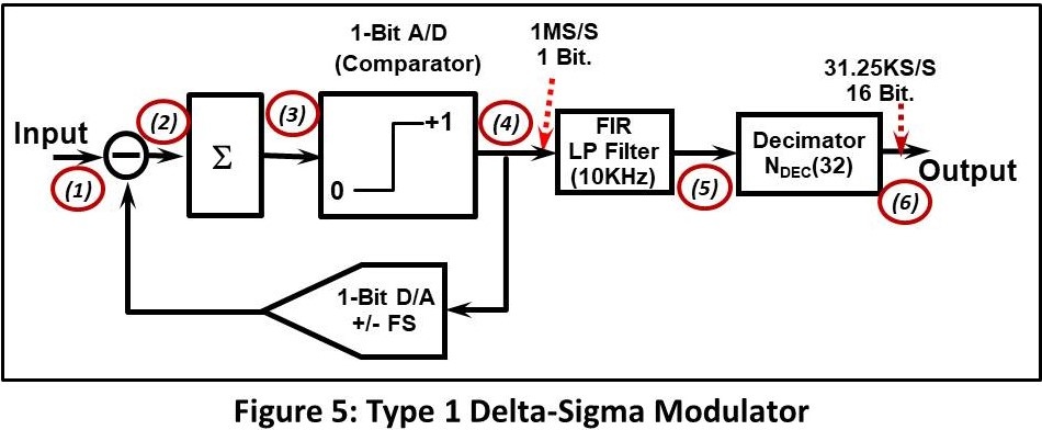
Figure 6 shows what happens at the critical points (1, 4, 5, 6) in the process.
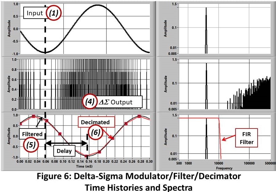
The upper frames show the input signal ((1) in Figure 3), a 4 KHz. sine wave, and its spectrum.
The output of the modulator ((4) middle frames) is a series of discrete values (1/0). When the input is low, the output is low (0) more of the time.. When it is high, the output pulse train is high (1) more. It’s a simple as that. Looking at the spectra we see that the output has the correct frequency component with a lot of high-frequency energy added by the modulator process. This noise pattern is predicted by the theory (Ref 1) but all we care about here is what to do about it.
The process is pretty obvious: Low pass filter the time history at just above our desired frequency range (FD) (5). Note that the low-pass filtering operation produces a significant delay.
Now we have a time history that is alias protected down to just above original desired bandwidth (F”OK”). Next, we decimate down to that sample rate (6).
The great thing about digital filters is that we can make them about any shape we want. More importantly for this discussion, we can make them pretty close to ideal (~square). Other advantages are that they are completely repeatable and are inexpensive (free?).
We have several options for the low-pass filter. One is a digital emulation of analog filters.. an option that is available in some commercial offerings (Ref 2) to emulate heritage systems. However, as we saw in the previous blog, these analog filters produce distortions due to either amplitude non-uniformity, phase non-linearity, or both. For most applications, we have a better option.
Finite Impulse Response (FIR) or Convolution Filters
In a later blog, we will go over the technology required to design FIR filters. Here we will just discuss the basic concept and describe a design that is appropriate for sigma-delta data acquisition system use.
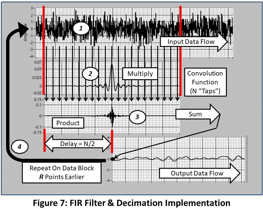
Convolution (Figure 7) is a simple, but very-compute intensive, process. The steps are:
- A block of N points of the input time history (1) is multiplied by the N-point convolution function (2) to produce the product (3).
- The N points in the product (3) are summed to produce a single point in the output (4).
- The operation is repeated on the input block offset forward by the decimation ratio (R) points. This provides the needed down-sampling (decimation) process.
So, the production of each point in the output requires N multiplies and N adds. A lot of work.. That is what Digital Signal Processors (DSPs) do well.
A cool feature of this operation is that the Decimation process is carried out at the same time as the filtering. The input data pointer is shifted forward by the decimation factor R at each step (32 in the example above).
The “buzz word for the size of the convolution filter is the numbed of “Taps”.
Obviously, the fundamental trick in the strategy is to come up with the convolution function that produces our desired filter characteristic. There are a variety of methods that we will discuss in a future blog. Here we will just show the result: the fllter used in the earlier example.
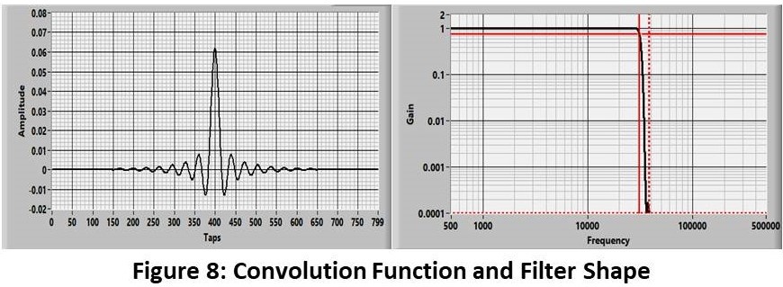
Figure 8 shows the filter shape that is produced with an 800-tap (N) convolution function. It has a cutoff frequency of 31KHz. and rolls off to 10,000/1 attenuation at ~ 38KHz. (A ratio of ~ 1.22).
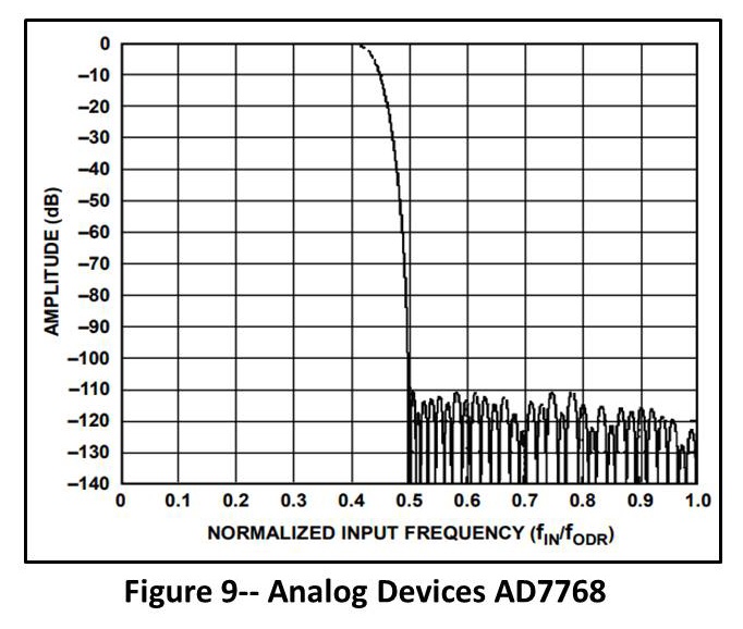
The filter in real Sigma Delta configurations (Example shown in Figure 9) is significantly sharper than this producing more out-of-band attenuation and/or better cutoff-frequency ratio. This is done with multiple FIR stages. Needless to say, the design is carefully held close to the chest of the vendors.
The oversampling/Sigma Delta filtering process produces an almost-ideal solution to the alias-protection process. Features include:
- Essentially flat pass-band response.
- Linear phase/constant delay.
- Excellent rejection of out-of-band response.
- Essentially perfect day-to-day and channel-to-channel matching.
Recap
This is the last of a blog set that discusses the effects (good and bad) of the solutions available for the handling of the aliasing problem in digital data acquisition.
-
Is Your Data Acquisition System Telling You The Truth? Discussed the fact that different data acquisition strategies produced different (but, in some cases, equally valid) results.
-
How Fast Must We Sample? Discussed the aliasing problem and how Shannon’s theorem answers some of the mysteries involved in digital acquisition.
-
Sample Rate: How to Pick the Right One continued the aliasing discussion and described the process required to estimate the required sample rate for different anti-alias-filter strategies.
-
Which Anti-Alias Filter is Best? attempted to answer the universal question in its title. The pros and cons of the different filter choices were hashed out and my opinion was expressed.
-
Analog Filter Design discussed the basic concepts and one of the strategies used to design analog filters.
-
This entry describes the concept of hybrid analog/digital, oversampling/sigma-delta filter designs.
Future blogs will discuss my view of other aspects of the digital data acquisition process. Potential topics include:
- Testing and verifying the performance of your present, or potential, data acquisition system.
- Strategies for selecting the optimal-gain/signal-range options.
- Strategies for the evaluation of potential damage from shock/impact events.
- Resampling: Tools that can be used to change the sample rate from the acquired value to a higher or lower speed.
- Transfer-function Compensation: The process we might use to make data acquired with one filter (Butterworth?) look like it was acquired by another (sigma-delta?).
- Design of FIR filters with arbitrary/non-classical characteristics.
- Your ideas are solicited.
These References will give you more information and, in some cases, a different view of the hybrid filtering operation.
- http://www.analog.com/en/technical-articles/behind-the-sigma-delta-adc-topology.html
- https://www.maximintegrated.com/en/app-notes/index.mvp/id/1870
- https://www.intersil.com/content/dam/Intersil/documents/an95/an9504.pdf
- http://www.rpi.edu/dept/ecse/rta/LMS/Delta-Sigma_ADCs.pdf
- http://www.beis.de/Elektronik/DeltaSigma/DeltaSigma.html
- http://www.analog.com/en/design-center/interactive-design-tools/sigma-delta-adc-tutorial.html
- https://en.wikipedia.org/wiki/Analog-to-digital_converter
- https://en.wikipedia.org/wiki/Delta-sigma_modulation
- http://www.analog.com/en/landing-pages/001/glp1-precision-lfs-sigma-delta.html
- http://www.analog.com/media/en/technical-documentation/technical-articles/ADI-data-conversion.pdf
Send a Comment or Question to Strether

One of the reasons I've been writing these blogs is to get a discussion going. Please reach out to me with any questions or comments you may have.
You can participate by:
- Entering comments/questions below in the Comments Section at the end of the blog. This will obviously be public to all readers.
- Contact me directly. I will respond privately and (hopefully) promptly. If appropriate, your question could be the subject of a future blog.
This blog is meant to be a seminar... not a lecture. I need your help & feedback to make it good!
Disclaimer
Strether has no official connection to Mide or enDAQ, a product line of Mide, and does not endorse Mide’s, or any other vendor’s, product unless it is expressly discussed in his blog posts.
Additional Resources
If you'd like to learn a little more about various aspects in shock and vibration testing and analysis, download our free Shock & Vibration Testing Overview eBook. In there are some examples, background, and a ton of links to where you can learn more. And as always, don't hesitate to reach out to us if you have any questions!